Category Modeling and Simulation of Aerospace Vehicle Dynamics

Flight Simulator

In today’s world of personal computers, everybody with a joystick has flown some kind of a flight simulator. They are so sophisticated that their flight dy­namics and cockpit layout approach the commercial product. However, the visual display confines the experience to a two-dimensional projection of the view out the window.

Workstation simulators are the elder cousins of the gaming simulator. With more computer power they model with greater fidelity the dynamics of the airborne vehicles, the surrounding terrain, and the cockpit layout. Large CRT screens with stick, rudder, and throttle give the pilot a realistic environment, albeit confined to two-dimensional displays and visual sensory feedback only.

The ultimate flying experience, short of air time, is in the six-DoF cockpit simu­lator mounted on a motion platform with full-scale cockpit and three-dimensional visual cueing. These are the simulators for commercial and military air crew train­ing. They have detailed six-DoF flight dynamics, accurate displays, and tactile feedback.

For military applications, where “blue” engages “red,” at least two simulators are needed. In close-in-combat (CIC) training, the two sides must “see” each other to practice evasive maneuvers and missile firing tactics. Dome – or tent-like screens envelop the cockpits and give the pilot a three-dimensional, large field-of – view perspective. One of the issues, which I will address, is the integration of the missiles into the simulation experience. Fidelity of the missile simulation must be balanced with execution speed.

I will define some general terms of flight simulators before treating the individual topics. As reference, I recommend the book by Rolfe and Staples.1 If you want to spend a delightful week in Cambridge, Massachusetts, attend the Massachusetts Institute of Technology summer course on fundamentals of flight simulation.2

Definition: A flight simulation is the dynamic representation of the behavior of

a vehicle in a manner that allows the human operator to interact with the simulation.

The dynamics are modeled mathematically by Newton’s and Euler’s laws, whereas the immersion of the operator occurs by sensory stimulants. A flight simulation can mimic any manned vehicle, from single propeller-driven pleasure craft to hypersonic aircraft and spacecraft.

Definition: A model is a representation, physical or analytical, of the structure

or dynamics of a system or process.

A physical model could be a subscale model airplane or a joystick masquerading as the flight controls. We distinguish between tangible and recorded models. Tangi­ble models are the cockpit, controls, instruments, and simulator domes. Recorded models are airport scenes, terrain models, wind and gust profiles, and sound effects.

Analytical models are based on physical laws expressed in mathematical terms. Some examples are Newton’s and Euler’s laws, INS error model, aerodynamic forces, actuators, propulsion units, and seekers.

The facility that comprises the flight simulator consists of five major compo­nents (see Fig. 11.1): aircraft model, the mathematical model of aircraft dynamics; vision system, the scene feedback to the pilot’s eyes; motion system, the vestibu­lar feedback to the pilot’s ears and tactile senses; acoustic system, the acoustic feedback to the pilots’ ears; and instruments, cockpit dials and displays. The pilot, receiving visual, acoustic, and vestibular feedback, controls the aircraft with the help of the cockpit instruments. A major part of the facility is devoted to the faith­ful replication of those stimuli. Deleting the motion system and simplifying the vision system can attain significant cost savings. You can find these shortcuts in some military trainers like the F15 simulator with its emphasis on medium-range intercepts and, of course, in any of the workstation simulators.

Real-Time Applications

The last three chapters gave you the opportunity to execute three-, five-, and six-DoF simulations of aircraft and missiles in the so-called batch mode. You gave the computer an executable form of your simulation and waited until the output came back. As outside agent, you may have yearned to get into the simulation and become a part of its world. Flight simulators, hardware-in-the-loop facilities, and war gaming let you be submerged into their virtual environments. To make the human experience real, the simulations must run in real time or at least be phased by real-time events.

The modeling techniques you have acquired will serve you well in building real-time applications. Preferably, you first construct a batch simulation and then synchronize it with a clock for real-time execution. You will have to balance model fidelity and execution time for best performance on your equipment.

Real-time simulations play a part at all levels of the simulation hierarchy. Re­call from Chapter 1 the pyramid of modeling hierarchy. At the foundation lie the engineering simulations, modeling systems, or subsystems with great fidelity, ffardware-in-the-loop HIL simulations are used to check out the performance of the system’s hardware and software before flight testing.

At the next higher level are the engagement simulations, which determine the effectiveness of aerospace vehicles. In military applications blue and red platforms may be engaged, firing projectiles or missiles at each other. The testing of equip­ment and air crew is carried out in air combat simulators, a special form of a flight simulator. In commercial applications the cockpit simulator is used to test handling qualities and to train airline pilots.

The upper two levels, called mission and campaign simulations, are tools for strategy or war games. What they lack in engineering detail they make up by a large aggregate of vehicles. As the multitude of entities interact, operational effectiveness is evaluated, and winning strategies are developed.

My purpose is to give you a taste of each of these categories. Drawing from my own experience, I selected topics from piloted simulators, HIL facilities, and war-gaming exercises. The genre however is so vast that you have to consult the specialty literature for particular applications.

SRAAM6

Подпись: Fig. 10.59 Ascent parameters of Fig. 10.58.

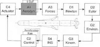
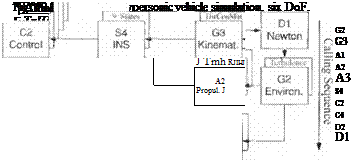
The SRAAM6 simulation models a generic short-range air-to-air missile. We encountered its five-DoF version already in Chapter 9. Now I present you with the flat-Earth, six-DoF benchmark version. By looking at the modules of Fig. 10.60, you can appreciate the complexity of this simulation. With nearly 6000 lines of FORTRAN code, it is the largest of all CADAC models. Actually, some of the modules are almost identical to the SRAAM5 versions. They are those forming

the navigation and guidance loop: Gl, SI, S2, S4, and Cl. Even the G2 and A2 modules can be adopted with minor modifications. However, the kinematic and dynamic modules are new and reflect the six-DoF implementation. They are summarized in Fig. 10.1. Let us briefly discuss the individual modules.

For the Gl Target Module target engagement scenarios are implemented. They are known by special designations, like Pre-Merge (shooter centered), One Cir­cle Fight, Two Circle Fight, Lufbery Circle, Target Centered Engagement, Chase Circle, Head-On Circle, and Twin Circle. You just need to set the flag MINIT and invoke the preprogrammed initial conditions for the target and the shooter aircraft.

For the G2 Environmental Module the ISO 62 standard atmosphere provides pressure, density, and temperature.

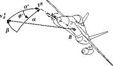
For the G3 Kinematics Module the incidence angles a’ and ф’ are calculated, and the quaternion methodology of Secs. 4.3.3 and 10.1.1 is employed to obtain the direction cosine matrix.

For the SI Seeker Module imaging IR sensors are the current state of the art of short-range air-to-air missiles. Although only generic data are used, the roll/pitch gimbals and the coordinate systems are quite realistic. You can find the description of the seeker in Sec. 10.2.6.

The S2 Air Intercept Radar is a simple kinematic model of an acquisition and tracking radar, located in the shooter aircraft. It acquires and tracks the target and transmits that information to the missile at launch and during an optional midcourse phase.

The S4 INS Module is used in midcourse only. The nine error state equations (three positions, three velocities, and three tilts) bring realism to the fly-out accu­racy. The derivation of the error equations is given in Sec. 10.2.4.

For the Cl Guidance Module a midcourse and terminal guidance phase is pro­vided. In midcourse a simple pro-nav law is implemented, whereas the terminal phase relies on the compensated pro-nav law of Sec. 10.2.5.

For the C2 Control Module, during separation from the launcher, only rate damping is provided. Thereafter, the proportional/integral autopilot of Sec. 10.2.2.4 provides rapid response to the guidance signals.

For the C4 Actuator Module four second-order actuators with rate and position limiters control the four fins. See Sec. 10.2.3.1 for details.

For the A1 Aerodynamics Module the aerodynamics are patterned after Eqs. (10.69) and (10.70). The coefficients are expressed in tables as functions of Mach and total angle of attack, for power on/off, and variable c. m. locations. The length of the missile is 2.95 m, and its diameter 0.1524 m.

For the A2 Propulsion Module the thrust of a single-pulse rocket motor is given as a table of thrust vs time with backpressure corrections. Vehicle mass, c. m., and MOI are updated. Launch mass is 91.7 kg, and the motor fuel is 35.3 kg.

The A3 Forces Module converts the aerodynamic coefficients to force and mo­ment vectors in body coordinates and adjoins the thrust component.

For the D1 Newton Module the translational equations of motion are formulated in body coordinates [see Eqs. (10.3) and (10.6)].

For the D2 Euler Module the rotational equations of motion (10.16) are solved in body coordinates.

For the G4 Impact Module the miss distance is calculated in the intercept plane. Figure 10.54 shows the details of a Monte Carlo run.

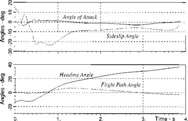
A typical engagement is shown in Fig. 10.61. With the shooter and target aircraft at the same altitude, the missile executes primarily a lateral maneuver, expressed by large excursions of the sideslip and heading angles.

SRAAM6

My mammoth chapter has come to an end. I did not expect you to study it line by line. Your professional specialization may have drawn you to the aerodynamic models, the autopilot implementations, the guidance laws, or the seeker mecha­nization. Some of you may have gone straight for the examples. Whatever your interest, you probably griped that your specialty is not adequately represented.

For you novices, unburdened by years of experience, I hope you sensed a cer­tain awe of the multidisciplinary challenge a six-DoF simulation poses. Learn by following in the tracks of others. Study the provided examples or other simulations and work the projects at the end of this chapter. Soon you will be the expert that others will consult in the pursuit of the perfect aerospace vehicle simulation.

References

‘Rolfe, J. M., and Staples, K. J., Flight Simulation, Cambridge Univ. Press, Cambridge, England, U. K., 1986.

2Zipfel, Peter H., “On Flight Dynamics of Magnus Rotors,” U. S. Army Technical Rept. 117, available at DTIC, ADA 716 345, Nov. 1970.

3“Department of Defense World Geodetic System 1984, Its Definition and Relationships with Local Geodetic Systems,” 3rd ed., NIMA WGS 84 Update Committee, NIMA TR 8350.2, Bethesda, MD, 4 July 1997.

4Torge, W., Geodesy, An Introduction, Walter de Gruyter and Co., Berlin, 1980.

5Britting, K. R., Inertial Navigation System Analysis, Wiley-Interscience, New York, 1971.

6AMTEC Corp., “Endo-Atmospheric Non-Nuclear Kill Simulation (ENDOSIM),” U. S. Army Strategic Defense Command, TR1158, TR1163, TR1161, Huntsville, AL, Aug. 1989.

’Jordan, W. E., “Simulation Models and Baseline Guidance and Control for Indirect-Fire Missiles with Strap-Down Inertial Guidance,” U. S. Army Missile Command, TR GR-76-41, Huntsville, AL, Jan. 1976.

8Savage, P. G., “Strapdown System Algorithms,” AGARD Lecture Series, No. 133, May 1984, p. 379.

9Stevens, B. L., and Lewis, F. L., Aircraft Control and Simulation, Wiley, New York, 1992, Eq. (1.3-6).

wLanchester, F. W., Aerodonetics, A Constable and Co., London, 1908.

11 Nielsen, J. N., Missile Aerodynamics, McGraw-Hill, New York, 1960.

l2Gentry, A. E., et al., “The Mark IV Supersonic-Hypersonic Arbitrary-Body Programs,” Air Force Flight Dynamics Lab., TR-73-159, Wright-Patterson AFB, OH, Nov. 1973.

13Williams, J. E., et al., “Missile Aerodynamic Design Method (MADM),” Air Force Wright Aeronautical Lab., TR-3109, Feb. 1988.

l4Magnus, A. E., and Epton, M. A., “PAN-AIR—A Computer Program for Predicting Subsonic or Supersonic Linear Potential Flows About Arbitrary Configurations Using a Higher Order Panel Method,” NASA CR-3251, Aug. 1982.

l5White, D. A., and Sofge, D. A. (ed.) Handbook of Intelligent Control, Van Nostrand Reinhold, New York, 1992, Chap. 11.

16Roskam, J., Airplane Flight Dynamics and Automatic Flight Controls, Vol. 1, Roskam Aviation and Engineering Corp., Lawrence, KS, 1979.

l7Britting, K. R., Inertial Navigation Systems Analysis, Wiley-Interscience, New York, 1971.

l8Widnall, W. S., and Grundy, P. A., “Intertial Navigation System Error Models,” Inter- metrics Rept. TR-03-73, May 1973, available from DTIC, AD 912 489L, Alexandria, VA,

l9Chatfield, A. C., Fundamentals of High Accuracy Inertial Navigation, Progress in Astronautics and Aeronautics, Vol. 174, AIAA, Reston, VA, 1997.

20Biezad, D. J., Integrated Navigation and Guidance Systems, AIAA Education Series, AIAA, Reston, VA, 1999.

2,Maybeck, P. S., Stochastic Models, Estimation, and Control, Vol. 1, Academic Press, New York, 1979.

22Stengel, R. F„ Stochastic Optimal Control, Wiley, New York, 1986.

23Hammersley, J. M., and Handscomb, D. C., Monte Carlo Method, Methuen and Co., London, 1964, reprint 1975.

24Zarchan, P, “Comparison of Statistical Digital Simulation Methods,” Guidance and Control Systems Simulation and Validation Techniques, AGARDograph No. 273, AGARD, 1988.

25Gelb, A., Applied Optimal Estimation, MIT Press, Cambridge, MA, 1974.

26Maybeck, P. S., Stochastic Models, Estimation and Control, Vol. 1, Academic Press, New York, 1979.

27Stengel, R. F., Optimal Control and Estimation, Dover, New York, 1994.

28Handbook of Geophysics and the Space Environment, U. S. Air Force Geophysics Lab., National Technical Information Center, ADA 16700, DTIC, Alexandria, VA, 1985.

29Von Karman, T, and Howarth, L., “On the Statistical Theory of Isotropic Turbulence,” Proceedings of the Royal Society of London A, Vol. 164, 1938, pp. 192-215.

3HDryden, H. L., “A Review of the Statistical Theory of Turbulence," Quarterly of Applied Mathematics, Vol. 1, 1943, pp. 7-42.

“Lumley, J. L., and Panowsky, H. A., The Structure of Atmospheric Turbulence, Wiley, New York, 1964.

■“Pritchard, F. E., et al., “Spectral and Exceedance Probability Models of Atmospheric Turbulence for Use in Aircraft Design and Operation,” U. S. Air Force Flight Dynamics Lab., Rept. AFFDL-TR-65F-122, Wright Patterson AFB, OH, Nov. 1965.

“Maybeck, P. S., Stochastic Models, Estimation, and Control, Academic Press, New York, 1979, p. 188.

“Nguyen, J. T., et al., “Simulator Study of Stall/Post-Stall Characteristics of a Fighter Airplane with Relaxed Longitudinal Static Stability,” NASA T. P. 1538, Dec. 1979.

Problems

10.1 GHAME6 flight control evaluation. The hypersonic NASA vehicle GHAME, modeled in GHAME6, has several control modes. You are to check out the dynamics of the open-loop and closed-loop response.

Task 1: Download from the CADAC CD the GHAME6 simulation and run

the test case INCLIMB. ASC. Try to maximize the terminal energy (altitude and velocity) at 1540 s flight time by modifying the trajectory profile. Plot your final trajectory (altitude, inertial velocity, Mach number, flight-path angle vs time) and record the end conditions of at least five trials in a table.

Task 2: Run GHAME6 without autopilot. Build the input file INOPEN. ASC

with the following modules: G2, ENVIRONMENT; G3, KINEMATICS; Al, AERODYNAMICS; A2, PROPULSION; A3, FORCES; D2, EULER; and Dl, NEWTON. With initial BALT = 15 km, DVBE = 720 m/s, and autothrottle set at 50 kPa, trim elevator DELEX to keep the vehicle with ±1000 m for 20 s.

Task 3: Determine the primary dynamic modes of the pitch, yaw, and roll

channels from Mach = 0.5 to Mach = 20 and plot the values.

Task 4: With the flight conditions of Task 2, execute a pitch doublet without

autopilot. Build the input file PITCH. ASC for a doublet of 5 deg and 10-s pulse width. Plot elevator deflection, pitch rate, and angle of attack vs time.

Task 5: Now, close the control loop by including the following modules: S4,

INS; C2, AUTOPILOT; and C4, ACTUATOR. Build input file INS AS. ASC for the yaw damper (SAS). Use ideal INS and maintain altitude with DELECX = 5 deg trim. Check the yaw damper with yaw-rate command pulse of 10 deg/s at 1-s pulse duration. Determine the best value for ZSAS. Why is the yaw rate response so sluggish? Plot yaw-rate command and response vs time.

Task 6: Check the roll controller. Build input file INROLL. ASC. Keep SAS,

and introduce a roll pulse of 10 deg and 4 s duration. Determine the best WRCL and ZRCL in conjunction with the best ZSAS damping. Plot roll command, roll rate, roll position, and aileron deflection vs time.

Task 7: Check the pitch acceleration controller. Build the input file

INACC. ASC. Keep SAS and engage the pitch acceleration controller. Initialize with 1.1 g, then introduce a 0.5-g incremental step command. Select through trial and error the best GAINP, WCLP, ZCLP, and PCLP Record these values, and plot acceleration command, achieved acceleration, angle of attack, and elevator deflection vs time.

Task 8: Finally, wrap around the acceleration loop the altitude controller. Build

the input file INALT. ASC. Maintain the initial altitude of 15 km, followed after 10 s by a altitude step command of 200 m increase. What are the best values for GAINALT and GAINALTD? Record these values and plot altitude, angle of at­tack, and elevator deflection vs time.

Task 9: Summarize your findings in a GHAME flight dynamics report. Show

all tables and plots.

10.2 Build a flight controller for the FALCON aircraft. The Falcon six – DoF simulation, available on the CAD AC C D, comes without autopilot. You are to transfer the flight controller from the GHAME6 simulation, integrate it into the FALCON6 simulation, and optimize the dynamic response.

Task 1: Familiarize yourself with the FALCON6 simulation, and run the in­

put file INPITCH. ASC. Plot elevator deflection, pitch rate, and angle of attack. Comment on the open-loop stability.

Task 2: Close the control loop with the C2 and C4 modules from GHAME6

SRAAM6 SRAAM6

and S4 module from SRAAM6. Add subroutine AIDER (derivative calculations) from GHAME6, A1 module to your FALCON6, A1 module. Ensure that all EQUIVALENCEd variables are consistent and that no errors remain after running MKHEAD3.EXE.

Build input file INYAW. ASC for the yaw damper (SAS). Use ideal INS, and check the yaw damper with a yaw-rate command pulse of 1 deg/s and 2-s pulse duration. Determine the best value for ZSAS.

Task 3: Check the roll controller. Build the input file INROLL. ASC. Keep SAS and introduce a roll pulse of 10 deg and 2-s duration. Determine the best WRCL and ZRCL together with the best ZSAS damping. Plot roll command, roll rate, roll position, and aileron deflection vs time.

Task 4: Check the pitch acceleration controller. Build file input INACC. ASC.

Keep SAS, and engage the pitch acceleration controller. Initialize with 1.1 g, then introduce a 0.5-g incremental step command. Select through trial and error the best GAINP, WCLP, ZCLP, and PCLP. Record these values, and plot acceleration command, achieved acceleration, angle of attack, and elevator deflection vs time.

Task 5: Wrap the acceleration loop around the altitude controller. Build the

input file INALT. ASC. Maintain the initial altitude of 1524 m, followed after 10 s by an altitude pulse command of 100 m and 20 s duration. What are the best values for GAINALT and GAINALTD? Record these values, and plot altitude, angle of attack, and elevator deflection vs time.

Task 6: Now build the heading controller, using the input file name IN­

HEAD. ASC. Make a 90-deg heading change and limit the roll angle to 70 deg. Determine the best FACTHEAD to reduce GAINPSI. Plot heading angle and roll angle with aileron and elevator deflections vs time.

Task 7: Let us climb with the aircraft. Build INCLIMB. ASC for the gamma-

hold controller and climb at 20 deg with a 10-deg heading change. Determine best PGAM, WGAM, and ZGAM. Plot heading and flight-path angles, with angle of attack roll angle, and all three control surfaces.

Task 8: Wind and nonstandard atmosphere are major disturbance factors. Build

the input file INWIND. ASC, based on INCLIMB. ASC for several conditions:

(a) Constant wind of 50 m/s from east.

(b) Shear wind from east: 1000 m, 50 m/s; 10000 nr, 100 m/s.

(c) Turbulence and shear wind with correlation length 150 m, sig = 2 m/s.

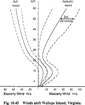
(d) Input mean wind in January at Wallops Island. Virgina (Fig. 10.45).

(e) Input a test atmosphere by increasing temperature by 10%, pressure by 10%, and reduce density by 10% from the standard atmosphere.

Choose variables that show the effect in each case and plot them vs time.

Task 9: Summarize your findings in a FALCON flight control report. Show

all tables, plots, and input files.

10.3 AGM6 air-to-ground missile. Convert the SRAAM6 air-to-air missile model into an unpropelled air-to-ground missile simulation AGM6, controlled by an autopilot, optimize the autopilot parameters, and document the results.

SRAAM6

Task I: Download the SKAAMb simulation from the CAD AC CD, run the

test cases, and plot selected parameters.

Task 2: Build the AGM6 simulation with a control loop only (no guidance).

Copy the following modules from SRAAM6: A3, G3, S4, C2, C4, Dl, D2, and adopt the G2 module from GHAME6. Download from the CADAC C D the AGM6 aerodeck and program the A1 module. Check carefully the interfaces, and make corrections as necessary. The utility MKHEAD3.EXE should diagnose no errors.

Task 3: Check the simulation first without control loop. Because the airframe

is aerodynamically stable, it should fly smooth ballistic trajectories. Excite the airframe with individual control inputs Sp, Sq, Sr at 1-deg magnitude and pulse width of 1 s. Do the transients damp out?

Task 4: First close the roll position and the pitch/yaw rate loops. Select optimal

values for the roll loop parameters WRCL and ZRCL. Adjust the rate autopilot parameter ZETLAGR for optimum performance.

Task 5: Now replace the rate loops by the acceleration autopilot. Adjust the

acceleration autopilot parameters WACL, ZACL, PACL for optimum performance.

Task 6: Study the effect of air turbulence on the AGM acceleration autopilot

using TRUBL = 150 m and TURBSIG = 3 m/s.

Task 7: Summarize the verification of your simulation in an AGM report.

Show the open- and closed-loop transient behavior about all axes and of all auto­pilot modes.

Simulations

The best way to learn the secrets of six-DoF simulations is by taking apart some well-written prototypes. In the early 1970s, when I was stranded at the White Sands Missile Range in New Mexico, 1 used the time to dissect my first missile six-DoF simulation. It was the spark that ignited the CADAC blaze.

There are a few good six-DoF simulations on the open market. If you can get your hands on one, study it diligently and learn by example. Here, I will describe briefly three prototypes based on the CADAC architecture. They have been mentioned throughout this chapter, and now the time has come to introduce them formally. The code is provided on the CADAC C D for your scrutiny.

9 G2 В G3 (ё A2 oo А1

Подпись:л>

■Є АЗ З D1 R D2

10.4.1 FALCON6

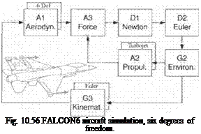
Let us start with a simple model. It is based on the description by Stevens and Lewis9 and the NASA database.34 Figure 10.56 depicts the seven essential modules of a six-DoF simulation: Newton’s and Euler’s equations with the aerodynamic and propulsive forces and the kinematic calculations. I will briefly describe each module.

For the Dl Newton Module the translational equations of motions [Eq. (10.3)] are solved with the flat-Earth assumption.

For the D2 Euler Module the rotational equations of motion [Eq. (10.18)] are tailored for aircraft with a cross product of inertia term. The angular momentum of the turbojet engine is also included.

For the G3 Kinematics Module the incidence angles a and /5 are calculated. The Euler angle rates are integrated to obtain the direction cosine matrix.

For the G2 Environment Module the ISO 62 standard atmosphere is imple­mented.

The AI Aerodynamics Module is patterned after Eqs. (10.61) and (10.62), but restricted to 0.6 Mach or lower.

For the A2 Propulsion Module the turbojet model of Sec. 9.2.2 applies here also. It calculates the thrust as a function of throttle setting, altitude, and Mach. It also includes a lag filter to model the spooling time delay.

The A3 Force Module combines the aerodynamic forces and moments with the turbojet thrust and readies them for the Newton and Euler equations.

The simulation does not have any controls. When you make a run, you may encounter an unstable region, and the trajectory will be cut short. I recommend you build your own autopilot, either by following Stevens and Lewis9 or working Problem 10.2.

10.4.2 GHAME6

Here we meet again the NASA GHAME that we employed in Chapter 8. Now it has fully blossomed into a six-DoF simulation with elliptical rotating Earth and a full suite of autopilot options. Figure 10.57 shows the modules and their special features. For a summary of the essential kinematic and dynamic equations, see Fig. 10.6.

Simulations

For the Dl Newton Module the translational equations of motion are formulated in inertial coordinates [see Eqs. (10.42) and (10.43)]. Vehicle position is converted to longitude, latitude, and altitude and velocity to geographic coordinates.

For the D2 Eider Module the rotational equations of motion (10.44) are expressed in body coordinates.

For the G3 Kinematics Module the incidence angles a and /І are calculated and the direction cosine matrix integrated from Eq. (10.47).

For the G2 Environmental Module the standard atmosphere ARDC1959 is im­plemented. Options are provided for tabular atmosphere and winds. The turbulence model of Sec. 10.3.3 is also coded.

For the AI Aerodynamics Module hypersonic aerodynamics are modeled ac­cording to Eqs. (10.65) and (10.66) and are based on NASA data.15

For the A2 Propulsion Module the combined cycle engine of Sec. 8.2.4 is mod­eled, consisting of a turbojet, ramjet, and scramjet phase. An autothrottle controls thrust to maintain constant dynamic pressure.

For the A3 Force Module the aerodynamic forces, moments, and propulsive forces are combined and expressed in body coordinates.

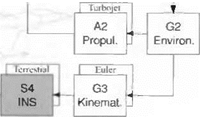
For the S4 INS Module the space-stabilized INS of Sec. 10.2.4 is implemented. Gyro, accelerometer, and gravitational perturbations are accounted for.

The C2 Control Module offers a variety of controllers: roll control, SAS, pitch acceleration controller, altitude hold, and both heading and flight-path-angle hold autopilots. Refer to Sec. 10.2.2 for a detailed description. All autopilot modes have aeroadaptive gains, derived by the pole placement techniques.

For the C4 Actuator Module second-order actuators with rate and position lim­iters control the elevons and rudder. See Sec. 10.2.3 for details.

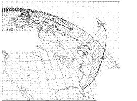
The CADAC CD has several test cases that you should exercise. Some results of the input file 1NCLIMB. ASC are displayed in Figs. 10.58 and 10.59. The run starts 3000 m above Cape Canaveral at a speed of Mach 0.75. Both the heading and flight-path-angle autopilots are engaged, and the autothrottle is set for 50 kPa dynamic pressure. After the climb-out at 20 and then 10 deg, the vehicle cruises at 30 km altitude until after 500 s it starts another shallow limb at 0.6 deg to top out at 40 km.

With the FALCON6 and GHAME6 code you have two simulations that cover the flight regimes of any aircraft over flat and elliptical Earth. Their aerodynamics

Simulations
is a function of the angles a and /3. We round out our collection by a missile simulation with polar incidence angles a’ and ф’.

Applications

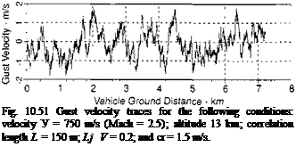
Подпись: Fig. 10.51 Gust velocity traces for the following conditions: velocity У = 750 m/s (Mach = 2.5); altitude 13 km; correlation length L = 150 m; Lj V = 0.2; and cr = 1.5 m/s.

The applications draw on the two CADAC simulations CRUISE5 and SRAAM6, the cruise missile and the short-range air-to-air missile. We will analyze the output

E

0)

о

3


Applications

Fig. 10.52 Medium roughness terrain, 30 Monte Carlo runs, mean and standard deviation.


Applications

using univariate and bivariate stochastic models. Of particular interest is the mod­eling of stochastic terrain, INS position error growth, impact accuracy, and launch envelopes. I will present only selected results; you can find more test cases on the CADAC CD.

In Sec. 9.3.3 I briefly described the random terrain, which models smooth, medium, and rough topography. A second-order power spectral density function is sampled for laying down the terrain ahead of the missile. Figure 10.52 shows the traces of 30 Monte Carlo runs and their univariate analysis, initiated at 3 s into flight. The mean altitude was set at 100 m. The mean of the stochastic traces deviates only slightly from this value. For an infinite number of runs, they would coincide. The spread of the tracks is characterized by the one-sigma band of ± 15 m. In CADAC the Monte Carlo technique is automated, and the univariate analysis is carried out by the utility program MCAP. EXE.

Another interesting study is the propagation of the INS position errors. In Sec. 10.2.4 I derived the error equations for space and terrestrial stabilized INS. Again making use of the CRUISE5 simulation with its terrestrial INS, Fig. 10.53 shows the 30 Monte Carlo replications before and after the start of the GPS up­dates. At launch the mean is slightly biased, and the one-sigma band is ±5 m. Starting with the first GPS update at 8 s into flight, the bias is eliminated and the stochastic error reduces to 1 m.

Bivariate distributions are usually related to miss calculations. They arise at aircraft landings, spacecraft docking, and missile intercepts. I use an air-to-air missile to illustrate the application.

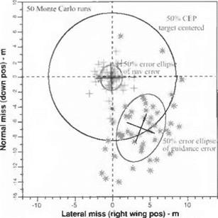
If you have solved Problem 4.11, you worked with the intercept plane that is used to record miss distance. Refer to the figure of Problem 4.11 to orient yourself. Fifty Monte Carlo shots were taken and recorded on the intercept plane in

Applications

Applications

Fig. 10.53 INS position error (north component) before and after GPS update, mean and standard deviation.

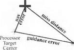
Fig. 10.54. The target aimpoint is centered at zero. As the right schematic indicates, miss distance is the vectorial sum of navigation and guidance errors. The crosses mark the point where the onboard processor places the target, and the stars are the actual impact points. On the intercept plane, the crosses cluster around the target, indicating that the navigation error is unbiased and equally distributed in both directions. Its 50% error ellipse is near circular. The impact points however are skewed by the 7-m bias and the 2:1 elliptical distribution. You as analyst will be asked the question whether the miss distance can be represented by the univariate CEP. How would you answer? The CEP is drawn, centered on the target, with a radius of 8 m. Is it an accurate measure of miss? I recommend that you give your customer the complete picture, explain the difference between univariate and bivariate distributions, and let him, according to his needs, make that judgement. The CADAC utility program KPLOT/BIVAR will help you prepare your presentation.

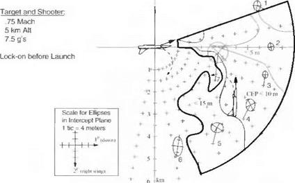
Figure 10.54 is based on a single engagement geometry between launch and target aircraft. It does not portray the performance of the missile under all possible launch conditions. The launch envelope of Fig. 10.55 provides that total picture. The scenario is a close-in engagement with both aircraft maneuvering at 7.5 g. The shooter (launch aircraft) is at the center of the envelope, whereas the target aircraft can be located anywhere, but maneuvering such that both canopies face each other. As long as the target is within the outer contour (at missile launch) it will be intercepted with the CEP indicated by the inner contours. To provide also the bivariate distributions, at selected points the bias and 50% miss ellipse are drawn at a magnified scale, as indicated in the box. For example, pick point 4 as the location of the target aircraft at missile launch. At intercept the CEP is less than 10 m with a bias of 8 m and an elliptical distribution about the mean as

Applications

Подпись: SIX-DEGREES-OF-FREEDOM SIMULATION 473

large!

Center


U’mile

Impact


Applications

Applications

Fig. 10.55 Launch envelope, shooter centered.

shown. Surveying the whole envelope, you see how bias and miss ellipse change with the engagement geometry.

Figure 10.55 packs a multitude of information into one graph. It can only be generated in reasonable time if the whole process is automated. The CADAC SWEEP methodology provides the wherewithal. You set up a Monte Carlo sweep run and let your computer chew on it over night. The next morning, you execute the SWEEP utility program with the IMPACT. ASC file from the previous night and produce a graph similar to my example. Your customer will be duly impressed.

Enough said of the elements of six-DoF simulations! I covered a smorgasbord of specialties, which, combined with the information of Chapters 8 and 9, should give you a broad taste of the variety of subsystems. Other specialties that I did not serve up you will have to find in the references. Unfortunately, much of the information lingers in unpublished notebooks of specialists. To round out this chapter, I will briefly describe three typical six-DoF simulations.

Turbulence

Atmospheric turbulence is air movement on a small scale. It is caused by the instabilities of pressure and temperature distributions in clouds, near the ground, and in the wind-shear regions of the jet stream. The fluctuations are time and space dependent. Because we cannot predict with certainty the behavior of the air molecules, we use statistical descriptors like standard deviation and power spectral density to classify the severity and spectral characteristics of turbulence.

For simulation purposes we make four assumptions that will ease the modeling task. The statistical properties of the turbulence are stationary (independent of time), homogeneous (independent of location in space), isotropic (independent of direction), and larger than the airplane (all parts of the airplane are equally af­fected). Two statistical representations are in good agreement with measurements: the von Karman29 and Dryden30 models. Although both yield similar results, the Dryden spectrum is preferable because it is easier to implement in simulations.

I will keep the modeling task simple. We limit ourselves to the one-dimensional Dryden spectrum and superimpose its turbulence on the air mass in the load factor plane of the aircraft or missile. (The load factor plane contains the total incidence angle a’). I pick this plane because our main interest is in the variability of the incidence angle and its effect on the vehicle.

Figure 10.46 shows the total incidence angle a’ as it relates to the angle of attack a and sideslip angle f3. We already encountered this spherical triangle in Fig. 3.19 with the corresponding angular relationship of Eq. (3.24). The aeroballistic wind axes A and 3A, which contain also the B body axis are embedded in the load factor plane. The transformation matrix [T]AB is given by Eq. (3.19).

Our goal is to express the movement of the turbulent air particles T wrt to the steady air mass A by the velocity vector vA and coordinate it in geographic axes [vA]G. The turbulence component r normal to the vehicle’s velocity vector v# in the load factor plane is expressed in the aeroballistic wind coordinates

[n^]A = [0 0 r]

With the two TMs [TAB and [T]BG we obtain the desired form

[vA]G = [T]bg[T]ab[va]A (10.140)

The entire movement of the turbulent air v B wrt Earth consists of the turbulence vA and the steady wind velocity v B. We program this superposition in geographic

Turbulence

Fig. 10.47 Aircraft entering a sine-shaped gust.


coordinates

[^]G = K]C + [^]C 00.141)

In Eq. (10.139) we used v^G as wind vector. If we want to include turbulence, we supplement it by [Vj]G and obtain the expanded expression

K]B = mBC{k£]c – (kA]c + Kf)} (10.142)

The vehicle’s velocity wrt air is now dependent on the geographic velocity Vg, the turbulent wind Vj, and the steady wind Уд.

Now we turn to the task of generating the velocity traces r based on the one­dimensional Dryden turbulence model. First, we need to convert the spatial pene­tration of turbulent air into a temporal process. Figure 10.47 shows an aircraft with velocity V preparing to fly into a turbulence field with sine-type vertical velocity distribution of length L. The spatial frequency of the wave is £2 = Ът/L. It takes an aircraft the time T — L/V to traverse the wave. The aircraft experiences the wave with the temporal frequency ш — 2л/T = 2л/(L/V).

Turbulent air consists not just of waves of one frequency but of a whole spec­trum. Their spectral density is modeled by Dryden’s function, expressed in the nondimensional frequency m — шТ — a>L/V

Подпись: (10.143)Подпись:a2 L 1 + Зпт2

2л V (1 + ти2)2

Turbulence

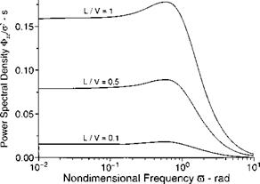
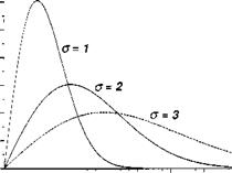
where a is the standard deviation of the turbulence in meters/second. The Dryden power spectral density function is shown in Fig. 10.48 for three L/V ratios. They

Turbulence

Fig. 10.49 Correlation length of turbulence.

peak near m = 0.6. For an aircraft traveling at V = 300 m/s and a turbulence correlation length L — 150 m, the peak frequency occurs at o> = 1.2 rad/s, not far removed from the pitch frequency of a large aircraft.

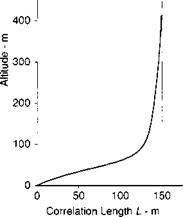
Correlation length L and standard deviation a are obtained from atmospheric measurements. Lumley and Panowsky31 give a detailed summary of L as a function of altitude. It is only near the ground, below 200 m, that it changes appreciably. At higher altitudes L maintains the constant value of 150 m length, as shown in Fig. 10.49.

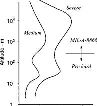
The intensity of the turbulence, represented by the standard deviation or, is a strong function of altitude. We follow Pritchard et al.32 up to 300 m and use the U. S. MIL Standard MIL-A-8866 for higher altitudes. Figure 10.50 depicts two curves.

Turbulence

Std. Deviation of Turbulence о – m / s

The medium profile represents the standard deviation at average gust speeds of 4 m/s, whereas the severe trace centers around 8 m/s. Notice the peak gust velocities in the jet stream of 8 ± 2.3 m/s, which is as much as 20 kn.

To generate time traces from the Dryden spectrum, we have to convert the power spectral density into a filter equation. Driving the filter with white Gaussian noise will produce the desired output. Spectral factorization (see Maybeck33) of Eq. (10.143) yields the transfer function of the gust variable r(s) over the white Gaussian noise vv(v)

r(s) lL/v 1+Уз (L/V)s ic(s)_CrV 2jt (L/V)2s2 +2(L/V)s + 1 For programming we convert the transfer function into its state-space form:

X]

0

і

X]

0

Xl

__ Lj

—– 1

<N

1

X2

+

.(r)2.

r (t) = a

"і V3-

Xl

v_

Xj

L/V

2jt

You can find these equations programmed in Module G2 of the CADAC GHAME6 simulation. A typical trace is shown in Fig. 10.51. This type of trace r(t) is inserted into the turbulence vector

[uj?]A = [0 0 r]

converted to geographic coordinates with Eq. (10.140), and combined with the wind velocity to be used for the incidence angle calculations in Module G3.

Winds and gusts are important feature of six-DoF simulations. They help us to investigate their effect on the performance, stability, and ride comfort of airplanes. You should be able to model steady winds and turbulence and use the provided data to conduct exploratory studies. For detailed analysis you should comply with the applicable industry standards and consult with the experts of your project team.

Winds

One of the effects studied in six-DoF simulations is the variability of the atmo­sphere. Air density may deviate from standard conditions, wind and wind shear may dislocate the vehicle, or atmospheric turbulence may shake up the passengers.

In Sec. 8.2.1 I introduced the standard atmosphere and its variations. The in­corporation of wind and turbulence requires the fidelity of six-DoF simulations. Three-DoF and pseudo-five-DoF simulations are inadequate because they do not model incidence angles based on the velocity vector but as output from the auto­pilot.

The air movement over the Earth can be divided into two components. The large – scale horizontal winds and the localized vertical gusts or turbulence. In simulations, tables represent winds as a function of altitude, direction, and magnitude, whereas turbulence, as a random phenomenon, is generated by a stochastic process. We shall discuss both phenomena.

To predict accurately the air movement over the globe is a complex problem. The mathematical model is formulated by partial differential equations and stochastic processes—techniques we would rather dodge. Fortunately, a large database exists of measured wind profiles over the Earth at all seasons, day and night. From this abundance you have to pick the winds that are appropriate for your study. If you have specific locations in mind, the National Oceanographic and Atmospheric Agency (NOAA) will be glad to supply you with archival information.

For sensitivity studies you can pick a particular wind profile that is representative of the winds your vehicle may encounter. A reasonable standard is the winds aloft Wallops Island, Virginia, where NASA’s Flight Center is located. Figure 10.45, derived from the Handbook of Geophysics,28 depicts the two extremes, the January and July winds. With little north-south activity it shows only the easterly and westerly components. Taken over many years, the mean winds are plotted against altitude. You can clearly see the jet stream bulges and the severe winds in the stratosphere. I also include a band, one standard deviation wide, to indicate the spread of the data around the mean wind.

You can use Fig. 10.45 or similar plots to define a single wind profile of projected severity, or you can establish an upper bound for winds occurring at a certain probability. For instance, the dashed lines on the right-hand side contain all westerly winds with probability 0.68. If you execute Monte Carlo runs, you can even have the simulation draw the wind profiles from a Gaussian distribution.

Altitude

Winds

In six-DoF simulations winds and gusts alter the incidence angles and thus change the aerodynamic forces and moments. The incidence angles are calculated from the velocity vector of the vehicle’s c. m. В wrt the air A, expressed in body coordinates ]B, [see Eqs. (3.20-3.23)]. To determine vB, we subtract the wind vector v д from the geographic velocity v § and introduce the body and geographic coordinates and their transformation matrix [T]BG

[vAB]B = [TfG([uf]G – [^]°) (10.139)

Ordinarily, the wind, assumed horizontal, is given by its magnitude Vw and direc­tion from north V’u,. Watch out however for the sign! A north wind blows the air from north to south. In geographic coordinates it has a negative 1G component. Therefore, the wind vector in geographic coordinates is determined by

[vaG = [-Vroc°s jrw – Vu. sin j/w 0]

In CADAC you use the weatherdeck to input winds in tabular form. Go to the G3 Module of the GHAME6 simulation and track down the code that implements Eq. (10.139).

Winds

Fig. 10.46 Total incidence angle a! in load factor plane.

Univariate Gaussian distribution

The simplest case is the one­dimensional output. Because we can assume the output parameters to be Gaussian distributed, our model is the univariate density function of the random variable x with mean цх and standard deviation ox:

1 (t-Д.;)2

p(x) =——- -=e (10.126)

Gx’Vl’K

Подпись: £"= Univariate Gaussian distribution Подпись: (10.127)

To calculate the mean ix and standard deviation ox from the output ensemble of your MC runs X], X2,…. x,-….. xn, you can use the following equation:

With these values the density function p(x) is determined, but it lacks intuitive­ness. If we integrate over the function, we get an easier-to-understand probability statement of the random variable x, namely, that the probability that x assumes the values between a and b equals the area under the density function:

P(a < x < b) = ( p(x)dx (10.128)

J a

Подпись: P (-z < — < +z V °x Univariate Gaussian distribution Подпись: л: ox Подпись: dt
Univariate Gaussian distribution Univariate Gaussian distribution
Univariate Gaussian distribution

You have heard of the so-called one-sigma, two-sigma, and three-sigma accuracy statements. For instance, what does it mean if the three-sigma navigation error is 50 m? With Eq. (10.126) substituted into Eq. (10.128), we can calculate the probabilities. Unfortunately, the value of the integral has to be obtained from tables. Instead of developing tables for every sigma and mean, a normalized table for sigma equals one, and zero mean is provided; it is called the normal table. Hence, we normalize the Gaussian density function under the integral by introducing t = x/ax and null the mean to get the probability areas between z = x/crx = ±1, ±2, ±3, ±4:

(10.129)

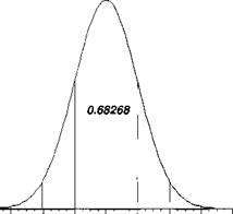
We look up the values of the integral between the z limits and record them in Table 10.2. For instance, the probability that the normalized random variable lies

Table 10.2 Multiples of standard deviations and associated probabilities

г

1

2

3

4

p

0.68268

0.95450

0.99730

0.99993

X = zo

1 a

2 a

3 a

4 G

0.4 и

Подпись: -5 -4 -3 -2 -1 0Подпись: 2 3 4Подпись: zПодпись:Univariate Gaussian distribution

Подпись: P(z)

0.3 –

0.2 – 0.1 – 0.0

between ±1 is 0.68268. With the same probability the random variable x lies between 1 x a. Figure 10.43 shows the normalized Gaussian density function. It is useful to visualize this so-called bell-shaped curve when you interpret your output. Applying Table 10.2 to our example, we expect that in 99.73% of occurrences the range error will be within 50 m.

Univariate Gaussian distribution

Instead of using the standard deviation to classify the range error, we can also ask the question: what is the 50% probability error bound.7 Starting with Eq. (10.129), we look for the integration bounds ±z that contain 50% of the area under the normal density function

From the normal table we interpolate for the value of 0.5 and receive г = 0.6745. For any distribution characterized by erv, we obtain, based on г = x/er,, the so – called range error probable (REP)

Подпись: (10.130)REP = zax = 0.6745ctv

Notice that the REP of 50% embraces smaller bounds than the one-sigma error, which occurs with the probability of 68.268% according to Table 10.2.

As an example, a fighter aircraft prepares to attack a target 3 km downrange. The pilot estimates that, given his one-sigma INS error of 100 m, he has a 50:50 chance to deliver the weapon within ±67.45 m of the required release point. The bomb itself has a ballistic error of REP = 50 m. Because both errors are statistically independent, they can be root mean squared together to provide the 50% probability that the bomb will land within V67.452 + 502 = ±84 m down – and up-range of the target coordinates.

The cross-range error or, as it is called, the deflection error probable (DEP) is defined in the same fashion. Given the lateral one-sigma error ery, then

DEP = 0.6745ery (10.131)

If the range and deflection errors are given by the univariate measures REP and DEP, the implicit assumption is made that the error distributions in the two directions are uncorrelated. You need to judge if this simplistic approach is adequate. When you analyze MC runs, you are more likely to find that the range and deflection errors are correlated, i. e., that they have a bivariate distribution. We now turn to discuss measures of accuracy for these two-dimensional situations.

10.3.1.2 Bivariate Gaussian distribution. Suppose you developed an air – to-ground guided missile simulation with many error sources and uncertainties. Now you execute MC runs and record the impact points in the x and у directions. From this two-dimensional data set*i, yu*2 , уг!• ■ ■ у і.. .’,xnyn, you calculate the means p. x, /лу and standard deviations ax, oy. You can adapt Eq. (10.127) to this process

Подпись: Mv Подпись: П En /=1 У І , Univariate Gaussian distribution Подпись: 2  2 Подпись: (10.132)

£"=і<л – РхУ

but you also have to check whether the data are cross correlated by calculating the covariance <r,,,

л у

Подпись:Y! i=i(xi – іххУуі – м>-)

Take note that the covariance is formulated without the square root. It has the squared units of x and y. Similarly, the variances of x and у are their standard deviations squared er2 and er2. The correlation coefficient can be calculated from the standard deviations and the covariance

Univariate Gaussian distribution Подпись: (10.134)

It assumes values between zero and one. Your data are uncorrelated if p = 0. In most cases they will be correlated, and you have to employ the two-dimensional Gaussian probability density function

as a model for the distribution of your data. Equation (10.134) portrays a bell­shaped surface over the x, у plane with its peak over the mean coordinates p. x and pty. A plane p(x, y) = const intersects the surface in the form of an ellipse. The

Univariate Gaussian distribution

Univariate Gaussian distribution

volume above the ellipse is the probability that a data pair x, у will appear within the confines of the ellipse. The variances and covariances establish a particular ellipse, which can be represented by the two-dimensional covariance matrix

It is a symmetric matrix, which can be diagonalized to obtain the major and minor axes of the ellipse. Once diagonalized in the new coordinate system (principal axes), the covariance is zero, and the data set has become uncorrelated.

When you analyze your impact points, it is helpful to draw so-called containment ellipses, centered on the mean values. They indicate to you the stretch of the data and the principal axes. The CADAC utility BIVAR, a subprogram of KPLOT, provides you with this display capability.

Sometimes, your customer may ask, “Could you boil down your misses into a single number?” Then you know that he is asking for the circular error probable CEP or the mean radial error (MRE). “No problem,” you say, “as long as you accept the simplifying assumptions.”

The definition of the CEP goes back to the times when the accuracy of rifles was determined by picking that circle on a paper target that contained 50% of the impact points. We take the mathematical approach and plot the radial distances r from the center as a histogram. If our simulation has enough noise sources with plenty of MC runs and the x and у dispersions are equal, we should see a density function similar to the Rayleigh distribution, also called the circular normal distribution. Its mathematical form is

Подпись: (10.135)p(r) = — e 2°r
W2

Подпись: 0.7Подпись:Подпись: 0.5Подпись: 0.4Подпись: 0.3Подпись: 0.2Подпись: 0.1Подпись: 0.0Подпись: 0Подпись: 2 3 4 5 6 7 8Подпись: rUnivariate Gaussian distributionP(r)

0.6

Univariate Gaussian distribution Подпись: ОГ2+ОГ? (10.136)

ar is calculated from the data set r, Г2, .. ., r,-, .. . r„ by an equation similar to Eq. (10.127).

Univariate Gaussian distribution Подпись: 0

Once the probability density function is given, we can calculate the 50% probability from the distribution integral taken from zero to the median m

Take the natural logarithm on both sides and solve for m:

2

Cn 1 — Hn2 ——– m = ar^2 ft 2 = 1.1774<тг

2<Tf

The CEP is the median m, i. e., the 50% probability that an impact point will occur within a circle of the radius,

CEP = .llAor (10.137)

I have raised several warning flags that you must recognize in order to properly interpret your results. If you have some insurance that your simulation produces Gaussian distributions, you can apply the Rayleigh function. However, the CEP is only a good single number if the x and у means are near zero and the impact pattern is skewed no more than 2:1. It is always advisable first to plot the mean center and the elliptical distribution before calculating a single CEP number. You can do this with the CADAC/BIVAR program that plots impact points, the mean, ellipses with their major axes, and actually two CEPs, the aimpoint (target)-centered and the mean-centered CEP.

The MRE is not to be confused with the CEP, although their numerical values differ only by 7%. Given a one-dimensional density function p(r), the mean is the expectation integral

/

30

rp(r)dr

•OO

The MRE is the expectation integral of the Rayleigh distribution with r the distance of the impact point from the target. Its solution is given in integral tables

fx r2 І7Ґ

E{r) = / — e 2r, r dr — ar /— = 1.253orr

J-oо V 2

Therefore the MRE of a radial distribution, which conforms to the Rayleigh func­tion, is

MRE = 1.253e>y (10.138)

Compare Eq. (10.137) with Eq. (10.138) and note the slight difference of the two accuracy measures.

We have reached the end of our short tour of Monte Carlo. Although you did not get any help for improving your chances at the roulette table, I hope you are equipped to conduct and analyze your MC simulations. The univariate measures of merit, REP, DEP, and standard deviation portray range and deflection accuracy or one-sigma errors of each INS channel. They are the easiest to analyze. More difficult are the bivariate measures of merit, particularly if the data are highly skewed. In that case we have to work with elliptical distributions. However, the desire to interpret the accuracy by a single number leads to the reduction of the bivariate data to a single radial distribution and the definitions of CEP and MRE. You will have to judge under what circumstances this shortcut is advisable. Some practical applications should help you to sharpen your tools.

Monte Carlo Analysis

If you know system engineers, you have heard them talk about Monte Carlo. They do not mean the picturesque city, nestled in the foothills of the Alps on the shores of the azure-blue Mediterranean, but they are referring to chance events; events that are too complex to model in all of their minute details.

We have already encountered some of them in the performance of INS and seekers. The complete error sources of INS sensors are so difficult to model that for system level analyses stochastic models like random walk, random bias, and white noise describe these uncertainties. Similarly, the IR sensor of Sec. 10.2.6 has a host of errors that model the imperfection of the electro/mechanical apparatus: aimpoint, jitter, bias, quantization, and blur of the focal plane array; rate gyros, gimbal noise, and bias of the mechanical assembly. Other uncertainties that affect the performance of an aerospace vehicle are airframe misalignments, erratic engine performance, and environmental effects of winds, gusts, and nonstandard atmo­spheric conditions. We already touched on nonstandard atmospheres in Chapter 8. In this section I will show you how to model winds and air turbulence, but first I must explain random events and their characterization.

What a throng of possible errors! It is the responsibility of the system engi­neer to define them mathematically and model them in the vehicle simulation. The stochastic nature of these errors produces random results. If the simulation were linear and the error sources were all Gaussian, the outcome would also be Gaussian. Then, the output covariances could be calculated directly from the input covariances. A single run of a so-called covariance analysis would suffice. How­ever, the world of aerospace vehicles can seldom be fully linearized. Our highly nonlinear five – and six-DoF simulations are witnesses to that fact. Therefore, many computer runs have to be executed, each time with a new draw from the random input. All output is then collected and analyzed.

The more runs you make, the closer to the truth you get; just like the more you frequent the casino of Monte Carlo the closer to bankruptcy you get—after all, the

casino has to make a profit for Prince Rainier of Monaco. The Monte Carlo tech­nique has its root in the Manhattan Project. It involved the simulation of the proba­bilistic phenomenon of neutron diffusion of fissionable material. Hammersley and Handscomb (H&H)23 give a readable summary of the 1964 status, and Zarchan24 emphasizes guidance applications. As H&H point out, the Monte Carlo method plays an important role in experimental mathematics. It addresses problems in statistical mechanics, nuclear physics, and even genetics, which are otherwise im­possible to solve. The specific Monte Carlo technique that applies to our problems is called the direct simulation method. Quoting from H&H, “… direct simulation of a probabilistic problem is the simplest form of the Monte Carlo method. It pos­sesses little theoretical interest and so will not occupy us much in this book, but it remains one of the principal forms of Monte Carlo practice because it arises so often in various operational research problems.” Could it be, because of its lack of mathematical sophistication, that it is so often called the brute force method?

There are three elements that you need to focus on: the validation of the sim­ulation, the input parameters, and the postprocessing of the output. If you read this chapter from the beginning and exercised some of the six-DoF examples, you have a good grasp of a typical simulation. As you build your own model, make sure that the level of detail is tailored to the particular problem. For trajectory studies you should concern yourself with aerodynamics, propulsion, winds, and nonstandard atmospheres; for targeting studies you have to add navigation and guidance uncertainties with realistic stochastic error models. Foremost, however, allow plenty of time and resources to verify your work. Test your simulation un­der various conditions, as you would test a prototype aircraft. Have other experts review your brainchild, and do not let fatherhood pride keep you from accepting corrections.

The input parameters must be accurate, but it is sometimes difficult to pick good values for random initializations and stochastic parameters. Because their statistical distributions assume infinite sample size, you are hard pressed to find sufficient data to support your choices. That deficiency is particularly evident for new concepts that have little test data for backup.

Output data are plentiful when you make Monte Carlo runs. As a rule, the more replications you execute the better the results, but, oh horror!, the more data you have to analyze. Hopefully, your simulation environment has some or most of these chores automated. CADAC Studio provides you with a host of statistical analysis tools, which you can tailor to your needs.

To apply these methods, you have to know the bare essentials of statistics, proba­bility, and random numbers. I assume that you have made their acquaintance so that I can concentrate here on the key elements of the Monte Carlo technique. Books by Gelb,25 Maybeck,26 or Stengel27 can help you overcome potential deficiencies.

The direct simulation technique of the Monte Carlo methodology addresses primarily questions of accuracy. How precise can an aircraft navigate over water, how close will the space shuttle come to the space station, or where will the missile hit the target? I will introduce you to some of the key concepts in accuracy analysis, like the circular error probable (CEP), error ellipses, and the practice of delivery accuracy investigations. Then, using CADAC-generated diagrams, I will demonstrate with practical examples the usefulness of the Monte Carlo method in establishing the performance of an aerospace vehicle.

10.3.1 Accuracy Analysis

Let us assume the aerospace vehicle design is well established, be it as a concept or as hardware, and a validated simulation is available. You, as system engineer, have to answer questions on performance and accuracy. With your powerful PC at your beckoning, you load the simulation, provide the input data, run repetitive runs, and then sit there, overwhelmed by the output. You probably have two questions: l) with the diversity of random input, what is the most likely statistical model of the output? and 2) how many runs are necessary for the output to be statistically significant?

Indeed, you may have a diverse array of input distributions. INS errors usually behave according to Gaussian statistics (normal distribution) and may be corre­lated in time (called Gauss-Markov processes). Similarly, seeker biases and noise behave mostly according to Gaussian and uniform distributions. More complex are the models of wind gusts that buffet your vehicle. Spectral densities with names like von Karman and Dryden have a long history in aircraft analysis. It gets even more complicated, however, for a terrain-following and obstacle-avoiding cruise missile. The terrain is modeled, unless you have actual data, by a second-order autocorrelation function, driven by white Gaussian noise, and you have to select three parameters to characterize the particular terrain roughness. Obstacles are generated by two stochastic functions: an exponential distribution that determines the distance to the next obstacle and a Rayleigh distribution that randomizes obsta­cle height. To get more insight, I recommend you scrutinize some of your favorite six-DoF models for their stochastic prowess or look at the CADAC simulations CRUISE5 and SRAAM6.

With that many random variables taken from different types of distribution, modified and filtered by linear and nonlinear dynamics, the question is what is the most likely distribution of the output parameters. The famous central limit theorem provides us with the answer. It asserts that the sum of n independent random variables has an approximate Gaussian distribution if n is large. This is good news indeed for our sophisticated six-DoF simulations. The more noise sources it contains, the more Gaussian-like the output will be. But what is enough? H&H state, “In practical cases, more often than not, n = 10 is a reasonable number, while n = 25 is effectively infinite.” Any respectable six-DoF simulation easily meets this condition. What a relief! We can use the well-established Gaussian statistical techniques to analyze the output.

With the output being Gaussian distributed, we can also answer the question of how many replications are necessary for a Monte Carlo analysis. It is based on the calculation of confidence intervals and their relationship to the standard deviation. Zarchan24 provides a graph that relates the number of sample runs to confidence intervals. For instance, if 50 Monte Carlo runs produced a unit standard deviation estimate, we would have a 95% confidence that the actual standard deviation is between 0.85 and 1.28. Increasing the run number to 200 would give us, at the same confidence level, an interval between 0.91 and 1.12. In my Monte Carlo studies I never use less than 30 runs (at 95%, 0.80 < a < 1.43) and increase them to 100 runs (at 95%, 0.89 < a < 1.18) if accurate estimates are essential.

Are you now anxious to analyze your output? We will discuss first the sta­tistical parameters of one-dimensional distributions, like altitude uncertainty or range error, the so-called univariate distributions, and then the two-dimensional
distributions, like ground navigation error or miss distance on a surface target, the so-called bivariate distribution.

Seeker kinematics

The main parts of an IR seeker are shown in Fig. 10.34. The optics, supported by the inner pitch gimbal, carries the focal plane array and is isolated from the support by the roll gimbal. To cool the detectors, the bottle contains pressurized nitrogen, which, when vented, cools and supplies the 70-80 К operating environment. The base of the sensor houses the electronics for the gimbals and the processor of the optical data. For an air-to-air application, the image processing can include target classification, aimpoint selection, and flare rejection. The main output of the sensor is the inertial LOS rate—target relative to the missile—expressed by the angular velocity vector of the LOS frame relative to the inertial frame.

Let us assail the coordinate transformations first. The mechanical roll and pitch gimbals orient the seeker head and its optics to the body frame. The associated head coordinates have their 1H axis aligned parallel to the optical axis and their 2H axis with the gimbal pitch axis. As you would expect, the seeker roll axis coincides with the body 1B axis. We build the transformation matrix [T]HB starting with the body axis, transforming it first through the roll gimbal angle фнв, and then through the pitch gimbal angle Qhb to reach the head axes, i. e.,

j// |яв_] Фнв_^в

Подпись: [T]HB = Подпись: cos 6цв sin 6HB sin фнв 0 cos фнв sin0Hs —COS6HB sin фнв Подпись: -&твНв cos фнв sin фнв cos QHB COS, фнв Подпись: (10.117)

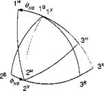
Figure 10.35 should help you visualize the two transformation angles. You can spot the two centerlines of the seeker and the missile, Iя and Is, respectively, separated by the angle вНв■ The gimbal transformation matrix (TM) is

Seeker kinematics

Fig. 10.35 Head wrt body transformation [T]HB.


Notice the difference of this roll/pitch TM and that of the pitch/yaw gimbals, Eq. (9.83). Both represent mechanizations with different limitations. The pitch/yaw implementation is limited in yaw to less than 90 deg—typically 63 deg—because of mechanical constraints. Our roll/pitch gimbal arrangement does not suffer these constraints, but has a singularity straight ahead, when the sensor points in the forward direction at any roll angle.

Because of this singularity, the processor implements a virtual gimbal transfor­mation, using the standard sequence of yaw and pitch (azimuth and elevation) from body coordinates to the so-called pointing coordinates. We have met this sequence several times. Please refer to Sec. 3.2.2 and in particular to Eq. (3.25) for details. The sequence of transformations is from body coordinates through the yaw angle 1f/рв

Подпись: [Т]РБ Подпись: cos 9PB cos фрв -sin iJrpB sin 9рв cos іf/рв Подпись: COS OpB sin JjpB COS фРВ sindpB sin 1j/рв Подпись: —sin врв 0 cos 9рв Подпись: (10.118)

and the pitch angle 9рв to the pointing coordinates, i. e., ]p. Its TM is

Seeker kinematics

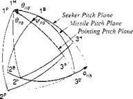
To compare the three coordinate systems, Fig. 10.36 delineates the body, head, and pointing axes with the angles of transformation, фНв, 9нв, and фнв, 9нв – You need to distinguish three different pitch planes. First, start with the missile pitch plane, subtended by Is and 3s, and roll through фнв to the seeker pitch plane Iя,

Seeker kinematics

Fig. 10.37 Spherical triangle and focal plane.

3й; second, start again with the missile pitch plane, but now yaw through іДрв to reach the pointing pitch plane lp, 3P.

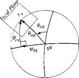
It is particularly informative to look down the nose of the missile and study the spherical triangle (Fig. 10.37) that encompasses the angles of both transformations. In it we see both the centerline of the missile 1B and that of the seeker head 1H. By Napier’s rule we can relate the pitch gimbal angle внв to the virtual gimbal angles

фрв, 9pb

внв = arccos(cos 9pB cos іДрв) (10.119)

as well as the roll gimbal angle

/ sin фрВ

Фнв = arctanl -—— ) (10.120)

V tan Орв )

When фрв = 0, then фив = 0; and when внв = 0, then фнв = 90 deg. Can you visualize the focal plane array centered and perpendicular to Iя?

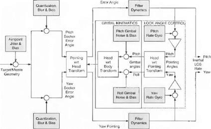
10.2.6.2 Seeker model. Having conquered the kinematics of the seeker, we can dig deeper and develop the mathematical seeker model. I shall break it into little bites as I have done before with the seeker in Sec. 9.2.5. But first, let us take the bird’s eye view of Fig. 10.38.

An IR seeker has two major functions: imaging and tracking. They are indicated by the bar on bottom of Fig. 10.38. The detectors of the focal plane array record the target image. By processing the gray shades of the image, the aimpoint is selected and its dislocation in the focal plane recorded as the error angle.

To be realistic, we have to include in our model some of the main error sources. They are identified in Fig. 10.38 by the shaded blocks. At the detector level a dynamic phenomenon called jitter can destabilize the image, and biases can be introduced by the optics. The finite number of elements affects the processing of the pitch and yaw error angles, and processing of the data introduces biases.

The tracking loop of the seeker consists of the mechanical gimbals, the LOS rate estimator, and several computational transformations. Some of the mechan­ical errors we consider are gimbal noise and biases and the instrument errors of

Seeker kinematics

Error Angle

I Aimpoml Displacement on Foca’ Plane | Tracking Loop. Gimbal Kinematics and LQS Rale Estimator-

Fig. 1038 Overview of the main elements of the seeker and their errors.


Подпись: 452 MODELING AND SIMULATION OF AEROSPACE VEHICLE DYNAMICS

the rate gyros. The dominant time lags are caused by the filtering of the LOS signals.

Let us follow the signal flow from left to right in Fig. 10.38. The model begins with the true missile-to-target geometry s bt■ Corrupting the target by jitter and bias creates the actual missile-to-aimpoint displacement Sab in head coordinates. Then the displacement is converted into pitch and yaw error angles and again diluted by quantization, blur, and bias uncertainties. Now the signals enter the computer­generated world of pointing coordinates and, after filtering, produce the inertial LOS rates in pointing coordinates as seeker output.

With the output generated, you may think that the seeker description is complete. But the all important seeker feedback loop still needs our attention. Through this loop the LOS rates, referred to the inertial frame, are transferred to the body frame by subtracting out the body rates. Then the pointing angles are converted into gimbal angle commands, which, after the gimbal noise and bias are added, establish the transformation matrix of the head to the pointing coordinates [T]HB. At this point the tracker loop is closed, and the transformation matrix [T]HB is available for converting the error angles from head to pointing axes.

After this overview let us explore the seeker model in detail. Again, we start at the left side of the schematic and discuss first the aimpoint model shown in Fig. 10.39. The true displacement vector of the missile c. m. В wrt the target centroid T is given by the simulation in local-level coordinates [s^r]1. It is transformed to the head axes and converted to the actual aimpoint [5дв]я by introducing the displacement vector [5дг]я that models the corruption of the true target point T by jitter and bias

[Тдв]Я = [5дг]Я — [^вг]Я

I lumped these errors together into the displacement vector [5дг]я and applied Gaussian noise and bias distributions to randomize the effects. Seeker specialists do not like such a top-level representation of a very complicated imaging process. Yet, if you are building a system simulation, you have to treat each subsystem with equal emphasis and have to compromise fidelity. Through cajoling, you may be able to convince your seeker expert to distill the imaging errors into this random vector [5дт-]Я.

Подпись: Aimpoint Jitter & Bias

The displacement on the focal plane is now converted into angles (see Fig. 10.40) and split into pitch and yaw error angle eY and eZ, respectively. At this point we

Seeker kinematics

introduce the processing errors of quantization, blur, and bias, which you have to extract from the seeker’s specification. I use random draws from a Gaussian distribution in radians to model their stochastic nature. The output of the image processor is sHY and sHZ.

Let us have a closer look at the focal plane in Fig. 10.41. Its center is the point H, which is also the piercing point of the Iя axis (see Fig. 10.37). The 2H and 3я axes complete the head coordinate system. On the focal plane is also located the aimpoint A, as determined by the image processor. The true displacement error, expressed in radians, is composed of the two error angles

[єШ_Iя = [0 sHZ -eHY] (10.121)

With perfect gimbals and processing this displacement would be the desired LOS rate output of the seeker. However, the tracker loop introduces additional errors caused by the rate gyros, the virtual gimbals (pointing axes), and the mechanical

3P

gimbals. Therefore, through the feedback loops the pointing axis 1p is displaced from the center of the focal plane 1H. The actual displacement, available for output processing, is the distance between the aimpoint A and the piercing point P of the 1p axis [eAPh. Our next task is to model this displacement.

The triangle of the three points A-H-P in Fig. 10.41 relates the measured value of [єАР]н to the true displacement [єАН]н and the pointing error [єРН]н

[єАР h = [є AH]H – [єРН] h (10.122)

The є should remind us that the values are small and expressed in radians. Although the true value is given by Eq. (10.121), the pointing error, which is a function of the mechanical and virtual gimbals, still needs derivation.

The two transformations. Eqs. (10.117) and (10.118). are combined to form the pointing to head coordinate transformation

[T]PH = T]PB[T]HB (10.123)

Now here comes the juggling! Associated with the pointing axis 1p and the head axis 1H are the unit vectors

ГрйҐ = [1 0 0] [7Г7]" = [1 0 0]

Their tip displacement is the pointing error

[єРН]н = [T]PH[Pl]p – [Іц]н (10.124)

If the two gimbal transformations were perfect, [T]PH would be unity and the point­ing error vanished. With Eqs. (10.121) and (10.124) substituted into Eq. (10.122), we have succeeded in modeling the measured aimpoint displacement on the focal plane array.

We transition now to the tracking loop by converting to pointing coordinates

[eAE]p = [T]ph[eAP]h (10.125)

and separating the measurements into pitch and yaw pointing error angles

ePY = —(eAP)p and ePZ — —{єАР)р

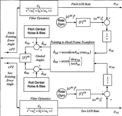
These angle errors are the input to the tracker loops. In Fig. 10.42 1 give you the entire tracking model so that you can follow in one graph the filtering, the body-rate compensation, the pointing angle generation, conversion to gimbal angle commands, and the gimbal mechanization.

The filters smooth the imaging and processing noise that come with the error angles before the LOS rates are sent out to the guidance computer. Flowever, the filtering causes time delays of the output signals. In effect, they are the dominant lags of the seeker. We use second-order transfer functions to model either a simple bandwidth filter or a sophisticated Kalman filter.

The output of the inertial LOS rates in pitch and yaw, ару and ri>z, respec­tively, are also the starting point of the feedback loops. Body rates from the INS rate gyros are converted to pointing coordinates and subtracted from the inertial LOS rates to establish the body-referenced LOS rates. Their integration leads to

Seeker kinematics

Fig. 10.42 Tracker loop.

the virtual gimbal angles фрв, врв, which are transformed by Eqs. (10.119) and (10.120) into the controls фнв, &нв of the mechanical gimbals. I have elected not to model the gimbal dynamics explicitly. State-of-the art technology delivers highly accurate mechanical devices, whose bandwidth is significantly wider than the filter response. Therefore, I account only for random noise and biases in the roll and pitch gimbals. The actual gimbal angles are фнв, бнв■ They determine the orientation of the focal plane array relative to the body frame, which is expressed mathematically by the transformation matrix

The tracker loop is now complete. The TM [T],m is combined with the pointing transformation [T]PB according to Eq. (10.123) to form the pointing wrt head TM [T]PH, which is used to convert the seeker error angles from head to pointing coordinates [see Eq. (10.125)].

Thanks for staying with me through this tour de force. You have mastered a difficult modeling task of a modern IR seeker, applying geometric, kinematic, and dynamic tools. The conversion to code is fairly easy with the provided equations. Yet, if you prefer, you can also use the code in the CADAC SRAAM6 simulation, Module S1. It is fully integrated into the short-range air-to-air missile. Its input file provides you with typical seeker parameters that you can use as a starting point for your simulation.

With this highlight we conclude the section of subsystem modeling of six-DoF simulations. You should have a good grasp of aerodynamics, autopilots, actuators, INS, guidance, and seekers. Supplemented by relevant material from the five-DoF discussion (Sec. 7.2), you should be able to model aircraft and missiles with six – DoF fidelity. If you need more detail, you can consult the experts. Assuredly, there are many more components of aerospace vehicles that we were unable to address. Unfortunately, the open literature is of little help. You will find contractor reports a proficient source of information, provided you can get access to them.

I hope you gained an appreciation of the modeling of aerospace systems. The best way to become proficient is for you to develop your own simulations. But first learn by example. Most of the examples I used have their counterpart in the software provided on the CADAC CD. I referred to them at the end of each section.

One more topic needs elaboration, which so far I have just alluded to: stochastic error sources for GPS, INS, seekers, and sensors and their effect on the performance of aerospace vehicles. With your curiosity aroused let us discuss these chance events.