Our heavyweight helicopter equal in the world does not have
In Rostov started production of the most load-lifting rotary-wing car The Russian holding «Helicopt[...]

Everything about aircrafts and helicopters. News and events in aviation worldwide. Civil, transportation, military helicopters and airplanes.

Everything about aircrafts and helicopters. News and events in aviation worldwide. Civil, transportation, military helicopters and airplanes.

Everything about aircrafts and helicopters. News and events in aviation worldwide. Civil, transportation, military helicopters and airplanes.

Everything about aircrafts and helicopters. News and events in aviation worldwide. Civil, transportation, military helicopters and airplanes.


The outlined geometry generator based on this explicit mathematical function toolbox allows for creating models for nearly any aerospace-related configuration The next step is to provide a w hole series of shapes w hich result from a controlled variation of a parameter subset kcyr with the option to create infinitesimally small changes between neighboring surfaces. This requires the introduction of а Чирсграгатсісг” t, its variation w ithin a suitable interval At and a general variation function f(t). Vanated parameters result then to
key fit) * *0,(0) ♦ /(f) Akeyt (71)
with Akey defined by the chosen extreme deviation from the starting values. Obtaining a series of surfaces calls for suitable computcrgraphic animation technology (119|. There are three major applications of introducing the 4th dimension (t) to the presented geometry generator for the development of design concepts:
Numerical Optimization
The success of optimization performing variations of a set of parameters small enough to enable the designer to control and understand the evolutionary process toward improved performance. but large enough to most likely include a global optimum, depends on selecting the parameters by knowledge based criteria. Simple first applications include the calibration of surface modifications as experienced from shock-frcc transonic design 1118). (120).
Adaptive Devices
A mechanical realization of numerical optimizing processes is the use of adaptive devices controlled by flow sensors [)2l|. Experiments arc needed for the development and understanding of the dynamics of such processes, as they are already routine for adaptive wind tunnel walls. Adaptive configuration shape simulation by the geometry generator will require a senes of shapes generated by selected functions equivalent to the mechanical model for clastic or pneumatic devices.
Unsteady configurations
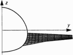
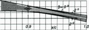
Finally there is time, the natural role of the superparameter t. Configurations may vary with time, especially if there is aeroclastic coupling between structure and flow. Periodically varying shapes arc generated to study the influence of moving boundary conditions on the flow. Modelling buffeting in the transonic regime is a wellknown goal, application of periodic geometries for a coupling of numerical structure analysis and CFD seems timely. Shape changes to model an adaptive helicopter rotor section with a sealed slat periodically drooped nose have been carried out and the results of unsteady Navicr Stokes analysis suggest a concept for dynamic stall control (122).
The usual way to connect two components is to intersect the surfaces Intersection curves arc found only by numerical iteration for non-invial examples. Most CAD systems perform such task if the data of different surfaces arc supplied. Here we stress an analytical method to find not only the juncture curve but also ensure a smooth surface across the components avoiding corners which usually create unfavorable aerodynamic phenomena. Sketched in Figure 61. this can be applied generally to two components Fj and Fs with the condition that for the first component one coordinate (here the spanwise y) needs to be defined by an explicit function у a F|(x. z), while the other component F may be given as a dataset for a number of surface points. Using a blending function for a portion of the spanwise coordinate, all surface points of Fj within this spanw ise interv al may be moved tow ard the surface F( depending on the local value of the blend-
 |
 |
ing function. Figure 61 shows that this way the wing root (Fj) emanates from the body (F|), wing root Fillet geometry can be designed as part of the w ing prior to this wrapping process. Several refinements to this simple projection technique have been implemented to the program.
Fuselage bodies, nacelles, propulsion ami tunnel geometries
This group of shapes is basically aligned w ith the main flow direction, the usual development is directed toward creating volume for payload, propulsion or. in internal aerodynamics (and hydrodynamics) the development of channel and pipe geometries. The parameters of cross sections arc quite different to those of airfoils: the quality of their change along a mam axis with constraints for given areas w ithin the usually symmetrical contour is the design challenge. Fuselages are therefore described by another set of “keys” which is defined along the axis. This axis may be a curve in 3D space, with available gradients providing cross section planes normal to the axis. For simple straight axes in the cartesian x-dircction key 40 defines axial stations just like key 20 defines spanwisc x-siations. With the simplest cross section consisting of supercllip – tic quarters allowing a choice of the half axes or crown lines and body pUnform. plus the expo-
 |
nents ( with the value of 2. for ellipses). 8 parameters (key 41 – 48) arc given (Figure 60). Basic bodies are described easily this way. with either explicitly calculating the horizontal coordinate y(x, z) for given vertical coordinate z, or the vertical upper and lower coordinate z(x. y) for given points у within the planform. at each cross section station x • const.
More complex bodies arc defined by optional other shape definition subprograms with additional keys (49 – 59) needed for geometric details. These may be of various kind but of paramount interest is the aerodynanucally optimized shape definition of wing-body junctures. In the following a simple projection technique is applied requiring only a suitable wing root geometry to be shifted toward the body, but more complex junctures require also body surface details to suitably meet the wing geometry.
Besides aircraft wings the tail and rudder fins as well as canard components are of course treatable with the same type of parameters and key functions. Highly swept and very short aspect ratio wing type components arc the pylons for jet engines mounted to the aircraft wing; they need to be optimized in a fiow critically passing between wing and engine. Generally any solid boundary condition to be optimized in flow with a substantial crossing velocity component is suitably defined as a spanwise defined component with a parameter set as illustrated for the wing.
|
|
|
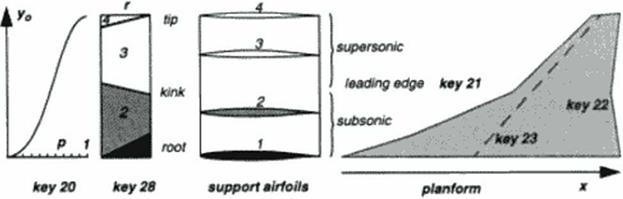
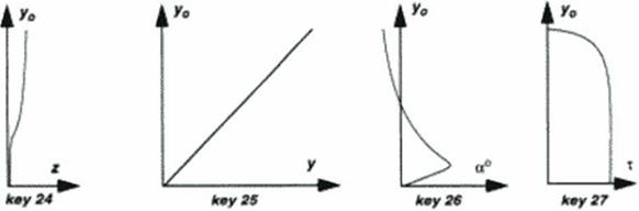
Figure 59 Wing parameter» and respective key numbers for section distribution, plunforni. an/dihedral, twist, thickness distribution factor and airfoil blending. |
Ain raft wings
Aerodynamic performance of aircraft mainly depends on (he quality of its wing, design focuses therefore on optimizing this component Using the present shape design method, we illustrate the amount of needed "key curves*’ along wing span which is inevitably needed to describe and vary the wing shape. Figure 59. The key numbers arc just identification names: span of the wing yQ in the w ing coordinate system is a function of a first independent variable 0 < p < 1. the curve y0(p) is key 20. All following parameters arc functions of this wing span, planform and twist axis (keys 21-23), dihedral (24) and actual 3D space span coordinate (25). section twist (26) and a spanwise section thickness distribution factor (27). Finally we select a suitably small number of support airfoils to form sections of this wing. Key 28 defines a blending function 0 < r < 1 which is used to define a mix between the given airfoils, say. at the root, along some main wing portions and at the tip The graphics in Figure 59 shows how the basic airfoils, designed with subsonic or with supersonic leading edges, may be dominating across this wing. Practical designs may require a larger number of input airfoils and a careful tailoring of the section twist to arrive at optimum lift distribution, for a given planform.
Recent updates to the wing generation include a spanwise definition of the previously mentioned 10-25 airfoil parameters as additional key functions, replacing given support airfoils and the blending key 28. Because of an explicit description of each w ing surface point without any interpolation and iteration, other than sectional data arrays describing the exact surface may easily be obtained very rapidly with analytical accuracy.
Wings with high lift systems are created using multicomponent airfoils cither for unswept wings with simply their varied deflected 2D configurations as illustrated in Figure 57. or in the more practical case of swept components (Figure 58) rotation axes and flap tracks need to be described as lines and curves in 3D space The clean airfoil configuration of the sy stem is then changed observing the given 3D kinematics.
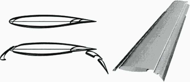
Lifting wings need mechanical control devices to vary their effective camber Geometrical definition of simple hinged and deflected leading and trailing edges arc defined by airfoil chord wise hinge locations and deflection angles. A more sophisticated mechanical flow control includes clastic surface components to ensure a certain surface smoothness across the hinge, such devices are called sealed slats and flaps (Figure 57). Spline portions or other analytical connection fits may suitably model any proposed mechanical device, an additional parameter is the chord portion needed for the elastic scaling
Multicomponent airfoils
While sealed flaps and slats arc suitable for supersonic w ings, the much more complicated multicomponent high lift sy stems have been developed for current subsonic transport aircraft In addition to angular deflection of slat and flap components, they require kinematic shifting devices housed within flap track fairings below the wing. For a mathematical and parameter-controlled description of slat and flap section geometries w ithin the clean airfoil, the richness of our function catalog provides suitable shapes and track curves for a realistic modelling of these components in every phase of start and landing configurations. Figure 58 illustrates a multicomponent tugh lift system in 2D and 3D.

|
|
|
In the ease of wing design we will need to include 2D airfoil shapes as wing sections, with data usually resulting from previous development. Having gone through CFD design and analysis, sometimes also through experimental investigations, these given data should be dense sets of coordinates without the need to smooth them or otherwise make geometric changes which are not accompanied by flow analysis. Airfoil research has its main applications in high aspect ratio wing applications in the subsonic and transonic flight regime. Supersonic applications with low – aspect ratio also need airfoils but their implementation to wing shaping requires mainly investi – gating the whole 3D problem. This leads to the option in the present geometry generator to provide again airfoil input data, but with only few coordinates: These can be used for spline interpolation in a suitably blown-up scale (Figure 56). For such few supports each point may take the role of an independent design parameter, wavy spline interpolation may be avoided if dislocations are small compared to distances to fixed points. Along one airfoil contour to be modified, portions of fixed contour with dense data distribution may be given while other portions may be controlled by only one or two isolated supports. This option was used in an early version of this geometry tool to optimize wing shapes in transonic flow (118].
|
Figure 56 Spline fit obtained for airfoil in blown-up scale with few support points |
Analytical sections and input for inverse design
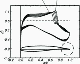
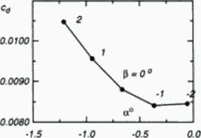
Spline fits arc well suited for redistribution of qualitatively acceptable dense data The possible occurrence of contour wiggles has restricted their use in the geometry tool discussed here to the abovcmcntioned option accepting external data, which is realistic for airfoils to be implemented in wing design. For a more independent approach we may ask for a more elegant analytical representation of wing sections, especially if these shapes still should be optimized. An important question arising is how many free parameters arc needed for representation of arbitrary, typical wing sections, with the shape close enough to duplicate CFD or experimental results of aerodynamic performance with reasonable accuracy Our successive refinement of airfoil generator subroutines using variously segmented curves as depicted in Figure 54 has shown that an amount of 10 to 25 parameters (numbers as listed in the table in Figure 54) may suffice for quite satisfactory representation of a given airfoil. The upper limit applies to transonic and laminar flow control airfoils with delicate curvature distribution as illustrated for a shock-free transonic airfoil. Figure 60 in chapter 7. where the influence of local curvature variations on the drag polar can be seen The lower limit seems to apply for simpler yet practical subsonic airfoils and for most supersonic sections.
With a library of functions applied to provide parametric definition of airfoils, another application of this technique seems attractive: new inverse airf oil and wing design methods need input target pressure distributions for specified operation conditions and numerical results arc found for airfoil and w ing shapes. The status of these methods is reviewed in the next book chapter Given the designer’s experience in aerodynamics for selecting suitable pressure distributions. choice of a few basic functions and parameters may provide a dense set of data cp(x/c) just like geometry coordinates arc prescribed, the amount of needed parameters for typical attractive pressure distributions about the same as for the direct airfoil modelling.
So far the geometry definition tool is quite general and may be used easily for solid modelling of nearly any device if a mathematically exact description of the surface, with controlled gradients and curvatures, is intended. In aerodynamic applications we w ant to make use of knowledge bases from hydrodynamics and gasdynamics. L e. classical airfoil and wing theory, as well as the classical results of slender body theory, transonic and supersonic area rule should determine the choice of functions and parameters. Surface quality should he described with the same accuracy as resulting from refined design methods outlined in the book chapter about the gasdynamic knowledge base. This is achieved by selecting suitable functions (G) when the key* curses axe subdivided into intervals defined by support stations. Slope and curvature control avoids the know n disadvantages of splines while at the same time the number of supports may be very low. if large portions may be modelled by one type of function.
In the process of making this generally described geometry tool to become dedicated geometry generator software for aerospace applications, a focusing on two main classes of surfaces has been found useful. There arc classes of surfaces which arc traditionally ‘spanwise defined’ and others arc ‘axially defined’. Lift-gciterating components like wings primarily belong to the first category w hile fuselages arc usually of the second kind. With this distinction having led to several practical versions of geometry generators, it should not be considered too dogmatically; especially novel configuration concepts in the high Mach number flight regime arc modelled without the above distinction as will be illustrated below, after describing the creating of conventional w ings and fuselages.
Aerospace applications call for suitable mathematical description of components like wings, fuselages, empennages, pylons and nacelles, to mention just the main parts which will have to he studied by parameter variation. Three-view geometries of wings and bodies are defined by plan – forms. crown lines and some other basic curves, while sections or cross sections require additional parameters to place surfaces fitting within these planforms and crown lines. Figure 54 shows a surface clement defined by suitable curves (generatrices) in planes of 3D space, it can be seen that the strong control which has been established for curve definition, is maintained here for surface slopes and curvature.
 |
Figure 55
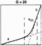
A set of functions Y(X) is suitably defined within the interval 0 < X < I. with end values at X. Y » (0. 0) and (1, 1). see Figure 53. We can imagine a multiplicity of algebraic and other explicit functions Y(X) fulfilling the boundary requirement and. depending on their mathematical structure. allow ing for the control of certain properties especially at the interval ends. Four parameters or less were chosen to describe end slopes (a. bland two additional properties (c^. fG) depending on a function identifier G. The squares shown depict some algebraic curses where the additional parameters describe exponents in the local expansion (G=1), zero curvature without <G=2) or with (G=20) straight ends added, polynomials of fifth order (G=6, quintics) and with square root terms (G=7) allowing curvatures being specified at interval ends. Other numbers for G yield splines, simple Bezier parabolas, trigonometric and exponential functions. For some of them a. b. cq and/or fG do not have to be specified because of simplicity, like G=4 which yields just a straight line. The more recently introduced functions like G=20 gisc smooth connections as well as the limiting cases of curves w ith steps and comers Implementation of these mathematically explicit relations to the computer code allows for using functions plus their first, second and third derivatives. It is obvious that this library of functions is modular and may be extended for special applications, the new functions fit into the system as long as they begin and end at (0.0) and (I, 1). a and b – if needed – describe the slopes and two additional parameters are permitted.
 |
 |
Y = Fq(a, Ь, Є$, 1q, X)
9.2.1 Curves
The next step is the composition of curves by a piecewise scaled use of these functions. Figure
54 illustrates this for an arbitrary set of support points, with slopes prescribed in the supports and curvature or other desired property of each interval determining the choice of function identifiers G. The difference to using spline fits for the given supports is obvious: for the price of having to prescribe the function identifier and up to four parameters for each interval we have a strong control over the curve. The idea is to use this control for a more dedicated prescription of special acrodynamically relevant details of airframe geometry, hoping to minimize the number of optimization parameters as well as focusing on problem areas in CFD flow analysis code development. Numbers serving as names ("keys*’) distinguish between a number of needed curves, the example shows two different curves and their support points. Besides graphs a tabic of input numbers is depicted, illustrating the amount of data required for these curves. Nondimensional function slopes a. b arc calculated from input dimensional slopes s( and s2. as well as the additional parameters Cq, f^ arc found by suitable transformation of c and f. A variation of only single parameters allows dramatic changes of portions of the curves, observing certain constraints and leaving the rest of the curve unchanged. This is the main objective of this approach, allowing strong control over specific shape variations during optimization and adaptation.
|
key |
u |
*2 |
e |
||||
|
1 |
d. d |
00 |
0. |
> |
б’.ЙГ |
4. |
6“ |
|
1 |
0.5 |
0.5 |
0. |
4 |
|||
|
1 |
1.7 |
0.8 |
025 |
6 |
0. |
0. |
■0.2 |
|
1 |
50 |
5° |
6 |
-0.8 |
-0.2 |
•0.2 |
|
|
1 |
7.5 |
to |
|||||
|
2 |
0.0 |
0.0 |
0. |
7 |
-0.5 |
4. |
0 |
|
2 |
1.0 |
-0.7 |
-0.5 |
20 |
***0.2 |
5. |
|
|
2 |
7.5 |
•1.3 |
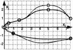 |
Figure 54 Construction of arbitrary, dimensional curves in plane (Xj, Xj) by piecewise use of scaled basic functions. Parameter input list with 2 parameters changed (shaded curves).