Our heavyweight helicopter equal in the world does not have
In Rostov started production of the most load-lifting rotary-wing car The Russian holding «Helicopt[...]

Everything about aircrafts and helicopters. News and events in aviation worldwide. Civil, transportation, military helicopters and airplanes.

Everything about aircrafts and helicopters. News and events in aviation worldwide. Civil, transportation, military helicopters and airplanes.

Everything about aircrafts and helicopters. News and events in aviation worldwide. Civil, transportation, military helicopters and airplanes.

Everything about aircrafts and helicopters. News and events in aviation worldwide. Civil, transportation, military helicopters and airplanes.


The fundamental form of expression for the coefficient of pressure applicable to two-dimensional compressible flow, with the frame of small perturbations, given by Equation (9.73), is:
Cp — -2 —.
p V«,
|
Therefore, in the present problem: |
||
|
1. Cp — —2hXe~Xz sin (Xx) |
for incompressible flow |
|
|
2hX 2. Cp ———– exp y/1 – Ml |
^ – X^J 1 – Ml j sin (Xx) |
for subsonic |
|
2hX 3. Cn = —, cos p V Ml – 1 ^ |
compressible flow |
|
|
X 1 & 1 |
for supersonic flow |
|
On the surface of the wall (г — 0) and above results reduce to: |
|
Cp — |
– 2hX sin (Xx) |
for |
incompressible flow |
(9.211) |
|
Cp — |
2hX —————- sin (Xx) |
for |
subsonic flow |
(9.212) |
|
л/1 – Ml |
||||
|
Cp — |
2hX ————- cosfXr) |
for |
supersonic flow. |
(9.213) |
|
vM -1 |
In the above solution we did not get f directly. The results are obtained from f’. If only Cp on the wall is needed, it is not necessary to find f, since the Cp on the wall is given by Equation (9.199).
2
Cp — — (f + g).
Vl
Usually, for aerodynamic applications, only Cp on the wall is necessary.
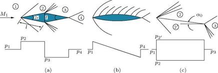
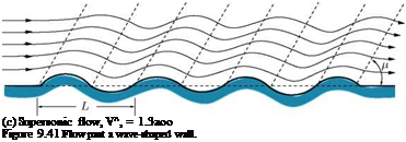
From the plots of incompressible, compressible subsonic and supersonic flow over wave-shaped wall, shown in Figure 9.41, the following observations can be made:
1. For Ml — 0, the disturbances die down rapidly because of the e~Xz term in Cp expression.
2. For Ml < 1, larger the Ml, the slower is the dying down of disturbances in the transverse direction to the wall.
3. For Ml — 1, the disturbances do not die down at all (of course the equations derived in this chapter cannot be used for transonic flows).
4. For Mto > 1, the disturbances do not die down at all. The disturbance can be felt even at to (far away from the wall) if the flow is inviscid.
Further, for equal perturbations, we have:
x — zJ M2 — 1 = constant.
As z ^ to,
• for Mto < 1, the disturbances vanish.
• for Mto > 1, the disturbances are finite and they do not die down at all.
Equation (9.212) is symmetric with respect to wall geometry and Equation (9.213) is asymmetric with respect to wall geometry. Therefore, when Cp is integrated along x, for Mto < 1, Cp becomes zero and for Mto > 1, the magnitude of Cp is > 0. In other words, in subsonic flow, the pressure coefficient is in phase with the wall shape so that there is no drag force on the wall, but in supersonic flow, the pressure coefficient is out of phase with the wall shape and hence there is drag force acting on the wall.
9.26 Summary
The incompressible flow is that for which the Mach number is zero. This definition of incompressible flow is only of mathematical interest, since for Mach number equal to zero there is no flow and the state is essentially a stagnation state. Therefore, in engineering applications we treat the flow with density change less than 5% of the freestream density as incompressible. This corresponds to M = 0.3 for air at standard sea level state. Thus flow with Mach number greater than 0.3 is treated compressible. Compressible flows can be classified into subsonic, supersonic and hypersonic, based on the flow Mach number. Flows with Mach number from 0.3 to around 1 is termed compressible subsonic, flows with Mach number greater than 1 and less than 5 are referred to as supersonic and flows with Mach number in the range from 5 to 40 is termed hypersonic.
A perfect gas has to be thermally as well as calorically perfect, satisfying the thermal state equation and at least two calorical state equations.
For a perfect gas, the internal energy u is a function of the absolute temperature T alone. This hypothesis is a generalization for experimental results. It is known as Joule’s law. We can express this as:
q = cvdT.
where cv is called the specific heat at constant volume. It is the quantity of heat required to raise the temperature of the system by one unit while keeping the volume constant.
Similarly the specific heat at constant pressure, cp, defined as the quantity of heat required to raise the temperature of the system by one unit while keeping the pressure constant. For p = constant, q = cpdT, therefore:
cpdT = (k + R) dT cp = k + R
cp — cv + R
or
This relation is popularly known as Mayer’s Relation.
Another parameter of primary interest in thermodynamics is entropy s. The entropy, temperature and heat q are related as:
q = Tds.
![]() The second law of thermodynamics assumes that the entropy of an isolated system can never decrease, that is
The second law of thermodynamics assumes that the entropy of an isolated system can never decrease, that is
When the entropy remains constant throughout the flow, the flow is termed isentropic Bow. Thus, for an isentropic flow, ds = 0.
This equation is often called the compressible form of Bernoulli’s equation for inviscid flows. The Bernoulli’s equation can be written as:
![]()
![]() = 0.
= 0.
This is a form of energy equation for isentropic flow process of gases.
For an adiabatic flow of perfect gases, the energy equation can be written as:
v22 vL
cpT2 + — = CpTi + —.
For air, with y = 1.4:
This maximum velocity, which is often used for reference purpose, is given by:
Another useful reference velocity is the speed of sound at the stagnation temperature, given by:
ao = J yRTo.
Yet another convenient reference velocity is the critical speed V*, that is, velocity at Mach Number unity, or:
V* = a*.
The one-dimensional analysis is valid only for flow through infinitesimal streamtubes. In many real flow situations, the assumption of one-dimensionality for the entire flow is at best an approximation. In problems like flow in ducts, the one-dimensional treatment is adequate. However, in many other practical cases, the one-dimensional methods are neither adequate nor do they provide information about the important aspects of the flow. For example, in the case of flow past the wings of an aircraft, flow through the blade passages of turbine and compressors, and flow through ducts of rapidly varying cross-sectional area, the flow field must be thought of as two-dimensional or three-dimensional in order to obtain results of practical interest.
Because of the mathematical complexities associated with the treatment of the most general case of three-dimensional motion – including shocks, friction and heat transfer, it becomes necessary to conceive simple models of flow, which lend themselves to analytical treatment but at the same time furnish valuable information concerning the real and difficult flow patterns. We know that by using Prandtl’s boundary layer concept, it is possible to neglect friction and heat transfer for the region of potential flow outside the boundary layer.
Crocco’s theorem for two-dimensional flows is:
It is seen that the rotation depends on the rate of change of entropy and stagnation enthalpy normal to the streamlines. Crocco’s theorem essentially relates entropy gradients to vorticity, in steady, frictionless, nonconducting, adiabatic flows. In this form, Crocco’s equation shows that if entropy (s) is a constant, the vorticity (?) must be zero. Likewise, if vorticity? is zero, the entropy gradient in the direction normal to the streamline (ds/dn) must be zero, implying that the entropy (s) is a constant. That is, isentropic flows are irrotational and irrotational Bows are isentropic. This result is true, in general, only for steady flows of inviscid fluids in which there are no body forces acting and the stagnation enthalpy is a constant.
The circulation is:
By Stokes theorem, the vorticity? is given by:
|
? = curl V
|
where? x, ?y, ?z are the vorticity components. The two conditions that are necessary for a frictionless flow to be isentropic throughout are:
1. h0 = constant, throughout the flow.
2. ? = 0, throughout the flow.
From Equation (9.33), ? = 0 for irrotational flow. That is, if a frictionless flow is to be isentropic, the total enthalpy should be constant throughout and the flow should be irrotational.
For irrotational flows (curl V = 0), a potential function ф exists such that:
The advantage of introducing ф is that the three unknowns Vx, Vy and Vz in a general three-dimensional flow are reduced to a single unknown ф.
The incompressible continuity equation v • V = 0 becomes:
or
v2ф = 0 •
This is a Laplace equation. With the introduction of ф, the three equations of motion can be replaced, at least for incompressible flow, by one Laplace equation, which is a linear equation.
The basic studies on fluid flows (Rathakrishnan, 2012) [2] say that:
1. For uniform flow (towards positive x-direction), the potential function is:
ф = Vx x.
2. For a source of strength Q, the potential function is:
, Q ,
ф = — ln r.
2n
3. For a doublet of strength p (issuing in negative x-direction), the potential function is:
p cos в
ф = ——— •
r
4. For a potential (free) vortex (counterclockwise) with circulation Г, the potential function is:
Г
ф = ^в•
2п
For a steady, inviscid, three-dimensional flow, by continuity equation:
V • (pV) = 0.
that is:
djpvxi d(pVy) d(pVz)
dx dy dz
 |
|
Euler’s equations of motion (neglecting body forces) are:
The basic potential equation for compressible flow is:
|
|
|
|
|
|
![]()
The difficulties associated with compressible flow stem from the fact that the basic equation is nonlinear.
The general equation for compressible flows can be simplified for flow past slender or planar bodies. Aerofoil, slender bodies of revolution and so on are typical examples for slender bodies. Bodies such as a wing, where one dimension is smaller than others, are called planar bodies. These bodies introduce small disturbances. The aerofoil contour becomes the stagnation streamline.
The small perturbation theory postulates that the perturbation velocities are small compared to the main velocity components, that is:
u V<x, v Vx, w V<x.
Therefore,
|
|
|
The equation valid for subsonic, transonic and supersonic flow under the framework of small perturbations with u « Vx, v « Vx and w « Vx.
This equation is called the linearized potential Bow equation, though it is not linear. For transonic flows (Mx & 1), the governing equation is:
|
|
The nonlinearity of this equation makes transonic flow problems much more difficult than subsonic or supersonic flow problems.
Fuselage of airplane, rocket shells, missile bodies and circular ducts are the few bodies of revolutions which are commonly used in practice. The governing equation for subsonic and supersonic flows in cylindrical coordinates is:
|
|
For transonic flow, this becomes:
Y + 1 1 1
■ ~r.— фх фхх + фгг +—— фг +—- 2 і
Vx r r2
For axially symmetric, subsonic and supersonic flows, фдд = 0. Therefore, the governing equation for subsonic and supersonic flows reduces to:
(1 — МТО)фхх + фгг + фг = °’
r
Similarly, the transonic equation reduces to:
Y + 1 1
—- — фх фхх + фгг +——- фг = °-
V» r
The small perturbation equations for subsonic and supersonic flows are linear, but for transonic flows the equation is nonlinear. Subsonic and supersonic flow equations do not contain the specific heats ratio Y, but transonic flow equation contains Y. This shows that the results obtained for subsonic and supersonic flows, with small perturbation equations, can be applied to any gas, but this cannot be done for transonic flows. All these equations are valid for slender bodies. This is true of rockets, missiles, etc. These equations can also be applied to aerofoils, but not to bluff shapes like circular cylinder, etc. For nonslender bodies, the flow can be calculated by using the original nonlinear equation.
Pressure coefficient is the nondimensional difference between a local pressure and the freestream pressure. The idea of finding the velocity distribution is to find the pressure distribution and then integrate it to get lift, moment, and pressure drag. For three-dimensional flows, the pressure coefficient Cp is given by:
Expanding the right-hand side of this equation binomially and neglecting the third and higher-order terms of the perturbation velocity components, we get:
For two-dimensional or planar bodies, the Cp simplifies further, resulting in:
This is a fundamental equation applicable to three-dimensional compressible (subsonic and supersonic) flows, as well as for low speed two-dimensional flows.
For bodies of revolution, by small perturbation assumption:
 u ( dR(x) Л
Vc„ У dx ) where R is the expression for the body contour.
An expression which relates the subsonic compressible flow past a certain profile to the incompressible flow past a second profile derived from the first principles through an affine transformation. Such an expression is called a similarity law.
Prandtl and Glauert have shown that it is possible to relate the solution of compressible flow about a body to incompressible flow solution.
The direct problem (Version I), in which the body profile is treated as invariant, the indirect problem (Version II), which is the case of equal potentials (the pressure distribution around the body in incompressible flow and compressible flow are taken as the same), and the streamline analogy (Version III), which is also called Gothert’srule.
Streamlines for compressible flow are farther apart from each other by 1 / 1 — M— than in incom
pressible flow.
The ratio between aerodynamic coefficients in compressible and incompressible flows is also
1Л/1 — Ml.
The freestream Mach number which gives sonic velocity somewhere on the boundary is called critical Mach number M’l. The critical Mach number decreases with increasing thickness ratio of profile. The P-G rule is valid only up to about MI.
In the indirect problem, the requirement is to find a transformation, for the profile, by which we can obtain a body in incompressible flow with exactly the same pressure distribution, as in the compressible flow. For this case:
That is, the lift coefficient and pitching moment coefficient are also the same in both the incompressible and compressible flows. But, because of decreased a in compressible flow:
Gothert’s rule states that the slope of a profile in a compressible flow pattern is larger by the factor 1 / y/1 — than the slope of the corresponding profile in the related incompressible flow pattern. But
if the slope of the profile at each point is greater by the factor 1 /^ 1 — Ml, it is also true that the camber (f) ratio, angle of attack (a) ratio, the thickness (t) ratio, must all be greater for the compressible aerofoil by the factor 1 / 1 — M—.
Thus, by Gothert’s rule we have:
![]() Zinc Mnc П. „ ,o
Zinc Mnc П. „ ,o
a f = – = GT—M„.
Compute the aerodynamic coefficients for this transformed body for incompressible flow. The aerodynamic coefficients of the given body at the given compressible flow Mach number are given by:
c± = c± = c^= 1
CP CL CM / Ml — 1
where Cp, CL and CM are at = V2 and C’p, C’L and CM are at any other supersonic Mach number.
For version II, we can write:
Cp _ Cl = Cm
Cp CL CM
Gothert rule for subsonic and supersonic flows gives:
We can state the Gothert rule for subsonic and supersonic flows by using a modulus: 11 — M^ For transonic flow:
( t 2/3
C’ ~ CL ~ Ы •
For subsonic flow:
Cp~cl~ (;)•
For supersonic flow:
Cp ~ CL ~ (O’
Transonic flow is characterized by the occurrence of shock and boundary layer separation. This explains the steep increase in CD at transonic range. We should also recall that the shock should be sufficiently weak for small perturbation. For circular cylinder this theory cannot be applied, because the perturbations are not small.
K = Мв,
where K is called the Hypersonic similarity parameter.
The presence of a small disturbance is felt throughout the field by means of disturbance waves traveling at the local velocity of sound relative to the medium. The lines at which the pressure disturbance is concentrated and which generate the cone are called Mach waves or Mach lines. The angle between the Mach line and the direction of motion of the body is called the Mach angle p.
at
sin p = — Vt
Shock may be described as compression front in a supersonic flow field and the flow process across the front results in an abrupt change in fluid properties. In other words, shock is a thin region where large gradients in temperature, pressure and velocity occur, and where the transport phenomena of momentum and energy are important. The thickness of the shocks is comparable to the mean free path of the gas molecules in the flow field.
is called the Prandtl relation.
In terms of the speed ratio M* = V/a*, we have:
This implies that the velocity change across a normal shock must be from supersonic to subsonic and vice versa. But, it can be shown that only the former is possible. Hence, the Mach number behind a normal shock is always subsonic. This is a general result, not limited just to a calorically perfect gas.
The relation between the characteristic Mach number M* and actual Mach number M is:
The Mach number behind is normal shock, M2, is:
![]() 1 +M2
1 +M2
YMf-V’
The density ratio across a normal shock is:
The pressure ratio across a normal shock is:
The ratio (p2 — p) /p = Ap/pi is called the shock strength.
The entropy change in terms of pressure and temperature ratios across the shock can be expressed as:
, T2 D, p2
S2 — ^ = Cp ln — — R ln —’
T p1
The changes in flow properties across the shock take place within a very short distance, of the order of 10—5 cm. Hence, the velocity and temperature gradients inside the shock structure are very large. These large gradients result in increase of entropy across the shock. Also, these gradients internal to the shock provide heat conduction and viscous dissipation that render the shock process internally irreversible. The flow process across the shock wave is adiabatic, therefore:
T02 = T01′
For a stationary normal shock, the total enthalpy is always constant across the wave which, for calorically or thermally perfect gases, translates into a constant total temperature across the shock. However, for a chemically reacting gas, the total temperature is not constant across the shock. Also, if the shock wave is not stationary (that is, for a moving shock), neither the total enthalpy nor the total temperature are constant across the shock wave.
For an adiabatic process of a perfect gas, we have:
r> 1 ^01
S02 – ^01 = R ln —- •
P02
Therefore, the entropy difference between states 1 and 2 is expressed, without any reference to the velocity level, as:
d і P01
s2 — s1 = R ln —— .
P02
The ratio of total pressure may be obtained as:
A compression wave inclined at an angle to the flow occurs. Such a wave is called an oblique shock. Indeed, all naturally occurring shocks in external flows are oblique.
The normal shock wave is a special case of oblique shock waves, with shock angle в = 90°. Also, it can be shown that superposition of a uniform velocity, which is normal to the upstream flow, on the flow field of the normal shock will result in a flow field through an oblique shock wave. All the streamlines are deflected to the same angle в at the shock, resulting in uniform parallel flow downstream of shock. The angle в is referred to as Bow deflection angle. Across the shock wave, the Mach number decreases and the pressure, density and temperature increase. The corner which turns the flow into itself is called compression or concave corner. In contrast, in an expansion or convex corner, the flow is turned away from itself through an expansion fan. All the streamlines are deflected to the same angle в after the expansion fan, resulting in uniform parallel flow downstream of the fan. Across the expansion wave, the Mach number increases and the pressure, density and temperature decrease.
Oblique shock and expansion waves prevail in two – and three-dimensional supersonic flows, in contrast to normal shock waves, which are one-dimensional.
The Mach number behind the oblique shock, M2, is related to Mn2 by:
![]() Mn2
Mn2
sin(e — в)
For a given initial Mach number M1, the possible range of wave angle is:
|
1 |
(1 ^ |
|
|
sin |
VM1У |
< в < 2 |
An important feature to be inferred is that the Mach waves, like characteristics will be running to the left and right in the flow field. Because of this the Mach waves of opposite families prevailing in the flow field cross each other. But being the weakest degeneration of waves, the Mach waves would continue to propagate as linear waves even after passing through a number of Mach waves. In other words, the Mach waves would continue to be simple waves even after intersecting other Mach waves. Because of this nature of the Mach waves, a flow region traversed by the Mach waves is simple throughout.
The 9~p~M relation of oblique shock is:
Oblique shocks are essentially compression fronts across which the flow decelerates and the static pressure, static temperature and static density jump to higher values. If the deceleration is such that the Mach number behind the shock continues to be greater than unity, the shock is termed weak oblique shock. If the downstream Mach number becomes less than unity then the shock is called strong oblique shock. It is essential to note that only weak oblique shocks are usually formed in any practical flow and it calls for special arrangement to generate strong oblique shocks. One such situation where strong oblique shocks are generated with special arrangements is the engine intakes of supersonic flight vehicles, where the engine has provision to control its backpressure. When the backpressure is increased to an appropriate value, the oblique shock at the engine inlet would become a strong shock and decelerate the supersonic flow passing through it to subsonic level.
The angle g is simply a characteristic angle associated with the Mach number M by the relation:
This is called Mach angle-Mach number relation. These lines which may be drawn at any point in the flow field with inclination g are called Mach lines or Mach waves. It is essential to understand the difference between the Mach waves and Mach lines. Mach waves are the weakest isentropic waves in a supersonic flow field and the flow through them will experience only negligible changes of flow properties. Thus, a flow traversed by the Mach waves does not experience a change of Mach number, whereas the Mach lines, even though they are weak isentropic waves, they will cause small but finite changes to the properties of a flow passing through them. In uniform supersonic flows, the Mach waves and Mach lines are linear and inclined at an angle given by g = sin-1 (1 /M). But in nonuniform supersonic flows the flow Mach number M varies from point to point and hence the Mach angle g, being a function of the flow Mach number, varies with M and the Mach lines are curved.
Even though all these are isentropic waves, there is a distinct difference between them. Mach waves are weak isentropic waves across which the flow experiences insignificant change in its properties, whereas the expansion waves and characteristics are isentropic waves which introduce small but finite property changes to a flow passing them.
It is important to note that, when we discussed about flow through oblique shocks, we considered the shock as weak when the downstream Mach number M2 is supersonic (even though less than the upstream Mach number M1). When the flow traversed by an oblique shock becomes subsonic (that is, M2 < 1), the shock is termed strong. But when the flow turning в caused by a weak oblique shock is very small, then the weak shock assumes a special significance. These kinds of weak shocks with both decrease of flow Mach number (M1 — M2) and small flow turning angle в can be regarded as isentropic compression waves.
![]() Y+ 1 M2 в
Y+ 1 M2 в
2 yMf—1 ‘
This is considered to be the basic relation for obtaining all other appropriate expressions for weak oblique shocks since all oblique shock relations depend on M1 sin в, which is the component of upstream Mach number normal to the shock.
Similarly, it can be shown that the changes in density and temperature are also proportional to в.
Compressions in a supersonic flow are not usually isentropic. Generally, they take place through a shock wave and hence are nonisentropic. But there are certain cases for which the compression process can be regarded as isentropic. This kind of compression through a large number of weak compression waves is termed continuous compression and these kinds of corners are called continuous compression corners. Thus, the geometry of the corner should have continuous smooth turning to generate a large number of weak (isentropic) compression waves.
In an expansion process, the Mach lines are divergent, consequently, there is a tendency to decrease the pressure, density and temperature of the flow passing through them. In other words, an expansion is isentropic throughout.
It is essential to note that the statement “expansion is isentropic throughout” is not true always. To gain an insight into the expansion process, let us examine the centered and continuous expansion processes. We know that the expansion rays in an expansion fan are isentropic waves across which the change of pressure, temperature, density and Mach number are small but finite. But when such small changes coalesce they can give rise to a large change. Therefore, it is essential to realize that a centered expansion process is isentropic everywhere except at the vertex of the expansion fan, where it is nonisentropic.
The expansion at a corner occurs through a centered wave, defined by a “fan” of straight expansion lines. This centered wave, also called a Prandtl-Meyer expansion fan, is the counterpart, for a convex corner, of the oblique shock at a concave corner.
It is known from basic studies on fluid flows that a flow which preserves its own geometry in space or time or both is called a self-similar Bow. In the simplest cases of flows, such motions are described by a single independent variable, referred to as similarity variable. The Prandtl-Meyer function is such a similarity variable.
The Prandtl-Meyer function in terms of the Mach number M1 just upstream of the expansion fan as:
The shock and expansion waves discussed in this chapter are the basis for analyzing large number of two-dimensional, supersonic flow problems by simply “patching” together appropriate combinations of two or more solutions. That is, the aerodynamic forces acting on a body present in a supersonic flow are governed by the shock and expansion waves formed at the surface of the body.
The only aerodynamic force acting on the diamond aerofoil is due to the higher-pressure on the forward face and lower-pressure on the rearward face. The drag per unit span is given by:
D = 2(p21 sin ё — p31 sin є) = 2 (p2 — p3) (t/2),
that is:
This gives the drag experienced by a two-dimensional diamond aerofoil, kept at zero angle of attack in an inviscid flow. This is in contrast with the familiar result from studies on subsonic flow that for two-dimensional inviscid flow over a wing of infinite span at a subsonic velocity, the drag force acting on the wing is zero – a theoretical result called d’Alembert’s paradox. In contrast with this, for supersonic flow, drag exists even in the idealized, nonviscous fluid. This new component of drag encountered when the flow is supersonic is called wave drag, and is fundamentally different from the skin-friction drag and separation drag which are associated with boundary layer in a viscous fluid. The wave drag is related to loss of total pressure and increase of entropy across the oblique shock waves generated by the aerofoil.
For the flat plate at an angle of attack a0 in a uniform supersonic flow, the lift and drag are computed very easily, with the following equations:
L = (p2 – pi) c cos a0 D = (pi – p2) c sin ao,
where c is the chord.
We saw that the shock-expansion theory gives a simple method for computing lift and drag acting over a body kept in a supersonic stream. This theory is applicable as long as the shocks are attached. This theory may be further simplified by approximating it by using the approximate relations for the weak shocks and expansion, when the aerofoil is thin and is kept at a small angle of attack, that is, if the flow inclinations are small. This approximation will result in simple analytical expressions for lift and drag.
At this stage we may have a doubt about the difference between shock-expansion theory and thin aerofoil theory. The answer to this doubt is the following:
“In shock-expansion theory, the shock is essentially a non-isentropic wave causing a finite increase of entropy. Thus, the total pressure of the flow decreases across the shock. But in thin aerofoil theory even the shock is regarded as an isentropic compression wave. Therefore, the Bow across this compression wave is assumed to be isentropic. Thus the pressure loss across the compression wave is assumed to be negligibly small. "
The above equation, which states that the pressure coefficient is proportional to the local flow direction, is the basic relation for thin aerofoil theory.
The CL and CD of the flat plate at a small angle of attack may be expressed as:
For a diamond wedge of chord c:
D _ 4s2
qic у7м2 – 1
or
![]() 4
4
л/м? -1 Vc
In the above two applications, the thin aerofoil theory was used for specific profiles to get expressions for CL and CD. A general result applicable to any thin aerofoil may be obtained as follows. Consider a cambered aerofoil with finite thickness at a small angle of attack treated by linear resolution into three components, each of which contributing to lift and drag.
By thin aerofoil theory, the Cp on the upper and lower surfaces are obtained as:
where yu and yl are the upper and lower profiles of the aerofoil. The profile may be resolved into a symmetrical thickness distribution h(x) and a camber line of zero thickness yc(x). Thus, we have:
where a(x) = a0 + ac (x) is the local angle of attack of the camber line and a0 is the angle of attack of the freestream and ac is the angle attack due to the camber. The lift and drag are given by:
The above two expressions give the general expressions for lift and drag coefficients of a thin aerofoil in a supersonic flow. In thin aerofoil theory, the drag is split into drag due to lift, drag due to camber and drag due to thickness. But the lift coefficient depends only on the mean angle of attack.
The fundamental equation governing most of the compressible flow regime, within the frame of small perturbations is:
(1 – MlAxx + ф« = 0.
This is elliptic for M, x) < 1 and hyperbolic for Mx > 1. There is hardly any method available for obtaining the analytical solution of the above equation for Mx < 1. But for Mx > 1, analytical solutions are available.
The governing equation for compressible subsonic flow is:
(1 – MlAxx + ф« = 0.
Solving as before, we get the result:
(x, z) =——– exp (- kzJ 1 – M21 cos (Xx).
V1 – Ml, ^ >
Hence, we have:
where в — cot Ц, — JM2 — 1.
The fundamental form of expression for the coefficient of pressure applicable to two-dimensional compressible flow, with the frame of small perturbations, is:
Cp — -2 —, p V ’
1. For Mto — 0, the disturbances die down rapidly because of the e~Xz term in Cp expression.
2. For MOT < 1, larger the MOT, the slower is the dying down of disturbances in the transverse direction to the wall.
3. For M,^) — 1, the disturbances do not die down at all (of course the equations derived in this chapter cannot be used for transonic flows).
4. For MOT > 1, the disturbances do not die down at all. The disturbance can be felt even at to (far away from the wall) if the flow is inviscid.
Further, for equal perturbations, we have:
x — z / M2 — 1 — constant.
As z ^to,
• for Mto < 1, the disturbances vanish.
• for Mto > 1, the disturbances are finite and they do not die down at all.
Exercise Problems
1. A flat plate aerofoil in a Mach 2 freestream experiencing a lift coefficient of 0.16 has an aerodynamic efficiency of 14.65, determine the drag coefficient and angle of attack.
[Answer: 0.0109, 3.97°]
2.
Show that for compressible flow of a perfect gas, the variation of total pressure across a streamline is given by:
where n is the direction normal to the streamline.
![]()
The nose of a cylindrical body has the profile R = ex3/2, 0 < x < 1. Show that the pressure distribution on the body is given by:
Estimate the drag coefficient for M = [ї and e = 0.1.
(Hint: For obtaining CD, use CDS(L) = Cp(x) S'(x)dx, where S(x) is the cross-sectional area of
the body at x and L is the length of the body.)
[Answer: CD = 0.0786]
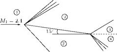
4. A slender model with semi-vertex angle в = 3° has to operate at M” = 10 with angle of attack a = 3°. What are the respective angles of attack required to simulate the conditions if a wind tunnel test has to be carried out at (a) M” = 3.0, в = 12° and (b) M” = 3.0, в = 3°?
[Answer: (a) 7.3°, (b) 16.3°]
5. A missile has a conical nose with a semi-vertex angle of 4° and is subjected to a Mach number of 12 under actual conditions. A model of the missile has to be tested in a supersonic wind tunnel at a test section Mach number of 2.5. Calculate the semi-vertex angle of the conical nose of the model.
[Answer: 19.2°]
6. Show that the results of the linearized supersonic theory for flow past a wedge of semi-wedge angle в may be put into the following similarity form:
![]() [(y + 1)m^1/3
[(y + 1)m^1/3
в2/3 where
x= M” -1______
X [в(у + 1)M”Г.
7. A shallow irregularity of length l, in a plane wall, shown in Figure 9.42, is given by the expression y = kx(1 — x/l), where 0 < x < l and k ^ 1. A uniform supersonic stream with freestream Mach number M” is flowing over it. Using linearized theory, show that the velocity potential due to disturbance in the flow is:
ф(Л’ y) = -—e k(x — ^ f1 — X i^’) ’
where в = M” — 1.
y.
Moo
![]() x
x
Moo
8. 
A two-dimensional wing profile shown in Figure 9.43 is placed in a Mach 2.5 air stream at an incidence of 2°. Using linearized theory, calculate the lift coefficient CL and the drag coefficient CD.
[Answer: CL = 0.06096 and CD = 0.04372].
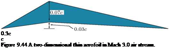
9. A two-dimensional thin aerofoil shown in Figure 9.44 is placed in Mach 3.0 air stream at an angle of attack of 2°. Using linearized theory, estimate CPu and Cpi.
[Answer:
Cpu = 0.211, Cpl = 0.046 (0 < x < 0.3c); Cpu = -0.1258, Cpl = -0.0551 (0.3c < x < c)]
10. The two-dimensional aerofoil shown in Figure 9.45 is traveling at a Mach number of 3 and at an angle of attack of 2°. The thickness to chord ratio of the aerofoil is 0.1 and the maximum thickness occurs at 30 percent of the chord downstream from the leading edge. Using the linearized theory, show that the moment coefficient about the aerodynamic center is -0.035, the center of pressure is at 1.217c and the drag coefficient is 0.0354. Show also that the angle of zero lift is 0°.
11. A two-dimensional wedge shown in Figure 9.46 moves through the atmosphere at sea-level, at zero angle of attack with = 3.0. Calculate CL and CD using shock-expansion theory.
[Answer: CL = —0.0388, CD = 0.02265]
12. Calculate the lift and drag coefficient experienced by a flat plate kept at an angle of attack of 5° to an air stream at Mach 2.3 and pressure 101 kPa, using (a) shock-expansion theory and (b) Ackeret’s theory.
[Answer: (a) CL = 0.1735, CD = 0.0152, (b) CL = 0.1685, CD = 0.0147]
13. Calculate the CL and CD for a half-wedge of wedge angle 5° kept in an air stream at Mach 2 and 101 kPa at (a) 0° angle of attack, (b) at 3° angle of attack.
[Answer: (a) CL = – 0.054, CD = 0.00497, (b) CL = 0.1778, CD = 0.01554]
14. If a2 = dp gives the local speed of sound, obtain the following forms of Bernoulli’s equation.
(a) a2 — + VdV = 0.
P
2a
(b) —– da + VdV = 0.
Y – 1
V 2 1
(c) y = (a0- a2).
The governing equation for this flow is:
(1 — МОТ)фХХ + Fz = °.
Solving as before, we get the result:
![]()
 |
|
ф(х, z) = — = exp — kz^J 1 — M2 cos(kx)
1 — M2a
Hence, we have:
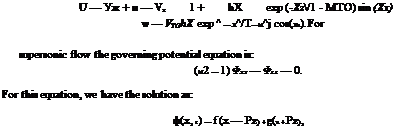
9.25.3 Supersonic Flow
For supersonic flow the governing potential equation is:
![]() (M2 — 1) фхх — Фzz = 0.
(M2 — 1) фхх — Фzz = 0.
For this equation, by Equation (9.196), we have the solution as:
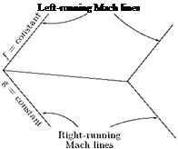
ф(х, z) = f (x — Pz) + g(x + Pz),
where в = cot Ц, = M2 — 1.
From the geometry of the problem under consideration, since the disturbances can move only in the direction of flow, there can be only left-running Mach lines, as shown in Figure 9.41(c). Therefore:
ф(х^) = f (x — Pz), g = 0.
 |
|
Hence, the perturbation velocity w on the wall is
Therefore:
The ф here is only the disturbance potential, and if the total potential is required, add (Vlx) to ф.
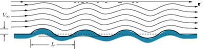
Consider a uniform flow of velocity Vx over a two-dimensional wave-shaped wall, as shown in Figure 9.41, with wavelength L and amplitude h.
Let the wall shape be defined by the equation:
zw = h sin(Xx). (9.201)
In Equation (9.201), subscript w stands for wall and X = 2л/L. Let us assume h ^ L, so that linear theory can be applied. By kinematic flow condition [Equation (9.68)], for z ^ 0, we have:
—- = —XXL – = hX cos (Xx). (9.202)
Lx, dx
Now, with this background, let us try to solve the governing equation for incompressible flow, compressible subsonic flow and supersonic flow.
9.25.1 Incompressible Flow
The governing equation for incompressible flow is the Laplace equation:
Fx + Фzz = 0.
This can be solved by expressing the potential function as:
Ф^, z) = F(x) G(z).
Solving by separation of variables, we get:
![]() ф^, z) = — Vxhe Xz cos (Xx).
ф^, z) = — Vxhe Xz cos (Xx).
 V
V
The potential function given by Equation (9.203) is only the perturbation potential. Obtaining the expression for ф, given by Equation (9.203), is left as an exercise to the reader.
Using Equation (9.203), we can easily get the resultant velocity U and perturbation velocity w as:
U = + u = VOT ^ 1 + hke~lz sin (kx) j (9.204a)
w = V(x, hke^kz cos (kx). (9.204i>)
From Section 9.10, by kinematic flow condition we know that:
|
w/Vx |
|
dz w |
|
u |
|
1 + — MX V |
|
(1 — в2 |
|
wdx. |
|
Vx dz |
|
Substituting for u and w from Equation (9.198), we obtain: |
|
Vxdz ^ 1 — y – (f’ + g) j = e(g’ — f’)dx Vxdz = e(g’ dx — f ‘dx) + e2(f ‘dz + g’dz) = в [ (g’dx + eg’dz) — (f’dx — ef ’dz) j = в (dg — df) , |
|
since: |
|
df df df = dx + — dz = f dx — ^f dz dx dz dg dg. . dg = dx + -2 dz = gdx + вg dz. dx dz |
|
Hence: |
|
dz = — (dg — df). V |
![]()
Integrating, we get the result:
This is the general solution of supersonic flow. Once the geometry is known, Equation (9.200) gives g and f and then from Equation (9.199) Cp and hence the lift and drag can be calculated. Therefore, in any problem if we are not interested in the geometry of the body present, then it is not necessary to find f and g. It is sufficient if f’ and g’ are found, to get the Cp, which is very much simpler.
Example 9.5
The upper and lower surfaces ofa symmetrical two-dimensional aerofoil are given by z = ±ex(1 — x/c)2, where c is the chord and e ^ 1. The aerofoil is at zero incidence in a steady supersonic stream of Mach number in positive x—direction. (a) Find the velocity components according to the linear theory in the upper region of disturbance. (b) Show that the drag coefficient of the aerofoil is given by:
![]() 8 e2
8 e2
15 .
Solution
(a) Given:
![]() Z = ±ex(1 — x/c)2.
Z = ±ex(1 — x/c)2.
The governing equation is:
2 д2ф д2ф
P dx2 — dZ2 =0
’(x, z) = f (x — Pz) for z > 0 (that is, above the aerofoil),
where P = JM^ — 1. On the upper surface, the boundary condition is:
(дФ L. ‘«- * (I)
With Equation (i), the boundary condition becomes:
 |
![]()
 |
Substituting X; in the equation for CD and simplifying, we get:
From the above discussions it is observed that:
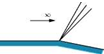
0. Disturbances and Mach lines can be produced only by boundaries.
1. Disturbances can travel only in the downstream direction.
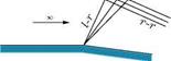
In Figure 9.39, we have shown that the characteristics of two families are independent of each other. This is because the geometries chosen are such that on one side of the boundary there is only one family of Mach lines. This is not the case always. In fact, in many situations of practical importance, the opposite characteristics will intersect each other as shown in Figure 9.40.
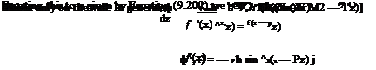
By knowing the type of Mach lines present in the problems, the equations can be suitably taken. From Equation (9.196), we have the potential function as:
ф(х, z) = f (x – Pz) + g(x + Pz),
where f represents the left-running Mach lines, on which g = 0 and g represents the right-running Mach lines, on which f = 0. The perturbation velocities are:
![]()
![]()
 |
|
 |
|
 |
|
дф
u = = фх = f + g
дх
дф
w ф = e(g – f)
dz
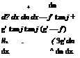
Then the pressure coefficient is given by Equation (9.73a) as:
u 2
= -2 V = – VT(f + g°-
![]()
|
|
|
![]()
![]()
|
||||||||||||||||||
|
 Moo
Moo