Category Aerodynamic measurements

If the velocity vector is at an angle в Ф 0 with the wire/sUpport plane (FigUre 3.18), the effective speed detected by the wire is

uf = ux + kuy + huZ

= U1 (cos2 a cos2 в + ksen2a + h1 cos2 asen2e)

where k = yaw factor, h = pitch factor.

Average valUes of h2 provided by the manUfactUrers are shown in the following table:

______________________________

Gold-plated probe 1.04

Fiber probe 1.20

In the particUlar case of planar flow (в = 0), one finds the sensitivity of the probe to the angle of yaw EqUation (3.17)

Uf (a) = U (cos2 a + k2sen2a) в = 0

Similarly the sensitivity of the probe at the pitch angle can be found by putting a = 0:

Uf (в) = U (cos2 в + h1sen1e) a = 0

The typical tool for determining both the unknown direction and absolute value of the velocity vector in a plane is the X-probe (Figure 3.19), consisting of two mutually perpendicular sensors, both at 45° with respect to the direction of the probe. The choice of these particular angles significantly simplifies the solution because the sine and cosine of 45° are equal and the sum of the angles formed by the velocity vector with the two wires is always 90°.

In the calibration phase, the probe is aligned with the stream and both wires are at 45° with respect to the direction of the velocity vector; the effective speed on each wire is

uiff=2^k )ui/

In the calibration phase, from the voltages measured on the two wires the corresponding values ucal1 and ucal2 are obtained. If in a test the speed is not aligned with the axis of the probe, the velocity components in the direction of the wires, u1 and u2 are derived from the following equations obtained by applying Equation (3.16) to the special case of the X-probe,

Figure 3.19

Probe syst.: x, у Wire syst.: 1,2

U = U1cosa1 + U2cosa2 V = U1sina1 – l^sinc^

in which case, since the two wires are mutually orthogonal, the component parallel to a wire is orthogonal to the other:

Finally, the components of the velocity vector in the direction of the pro­be and in the direction normal to it, u and v, respectively, are given by:

V2 ( + ) V2 ( )

U = — (l + U2 ) v = ~ (U1 – U2 )

If the stream direction is not normal to the sensor, the collected data are biased compared to those provided by the calibration. If the velocity vector lies in the wire/support plane, i. e. в = 0 in Figure 3.18, and if the angle from the normal to the wire is small, the component normal to the wire can be considered as the effective speed on the sensor

Ue[[ = Ucos а (3.16)

Decomposition of the velocity vector on the axes of the probe

For greater angles, the velocity component parallel to the sensor contributes, albeit with minor effectiveness, to cooling and that is why the more accurate Equation (3.17) must be used

Uf = U1 (cos2 a + ksen2a) (3.17)

The value of k2 (yaw factor) depends on the sensor type and on the length/diameter ratio of the wire and should be evaluated for each probe by varying the angle a in a known stream; alternatively, the average values provided by the manufacturers and listed below can be used:

If the probe is inclined with a known angle with respect to the direction of speed, the true value of the speed can be found from that measured by the probe by using, depending on the required accuracy, Equation (3.16) or Equation (3.17).

If the direction of velocity is unknown, it is not possible by Equation (3.16) or Equation (3.17) to obtain simultaneously the value and the

direction of speed (two unknowns from a single equation). It is necessary to use two sensors in two directions to obtain two independent measurements from which both unknowns can be calculated.

1.6.2 Calibration

To carry out any measure of average speed a calibration curve is needed. For measurements in gases at speeds between 10 and 100 m/s calibration can be made with reference to the difference in pressure read in a Venturi tube (a mini-subsonic wind tunnel) where the sensor is placed. For very low speeds, the use of a laminar flow tube is recommended. For higher speeds, a cylinder powered by compressed air and equipped with a set of interchangeable nozzles is used.

Obviously the accuracy of the calibration curve increases with the number of measured points. This involves a tedious procedure to be repeated frequently, even if the same probe is used, to check that the wear of the sensor or the presence of impurities in the stream have not altered the characteristics of the probe itself. The linearizer could alleviate the problem because it allows calibration by measuring only the voltage corresponding to the maximum speed.

In the classical analog anemometer, output voltage was measured with a DC voltmeter, that is a voltmeter with a considerable inertia, that even in the presence of fluctuations due to the turbulence of the fluid current, did not follow the fluctuations but showed an average value.

In modern anemometers, the signal passes through an analog/digital converter and is given as a large number, n, of numerical data representing the succession in time of voltage fluctuations. The average voltage is thus obtained by the equation:

– У, E

n

The non-linearity of the hot wire anemometer in the measurement of speed has been emphasized. The relationship between the electric power supplied to the sensor and velocity of the fluid stream that invests it, given in Equation (3.7), for a CTA (in which Tw = const, Rw = const), can be written as

E1 = ( + bJU){Tw – Ta)Rw = A + BU = E + BU (3.15)

where E0 is the difference of potential that occurs at U = 0.

To determine the average speed of the stream, it is only necessary to measure the average voltage output of the anemometer and use the cali­bration curve. But this is fully satisfactory only if the level of turbu­lence is low; if this level is high, due to the nonlinearity of the calibration curve, the average voltage does not match the average speed but a lower speed.

In order to linearize Equation (3.15), it is necessary to pass the output of the anemometer through an apparatus with a transfer function which is the inverse of King’s law. Consider:

EOM = k(En – C )m

where M, C and k are constants.

If the output voltage of the anemometer is replaced by Ein (Equation 3.15):

Eut = k(E0 + BU – C )m

Making C = 0: Eout = k(b4u)m

making m = 2 Eout = kB2U

But kB2 = K, then Eout = KU. In this way, the output of the linearizer is a voltage proportional to velocity.

Since the output voltage of the anemometer depends on the fluid stream temperature, Ta, this must be taken into account every time it varies during the test or between calibration and measurement, for
example, an increase in ambient temperature looks like a decrease in stream speed.

There are various methods for correcting temperature:

■ the temperature is measured separately and the data are corrected referring to a family of calibration curves plotted for different temperatures (Figure 3.17) or by using the theoretical equations of heat transfer;

■ using two active sensors operating at two different temperatures and making the difference between the output signals to obtain a signal independent of the stream temperature; in particular, the compensation sensor operates at low temperature and is therefore insensitive to velocity. The following equations can be written for the power outputs of the two sensors:

W = (+1*U){T – Ta) W2 = (+bU) – Ta)

W – w2 = (+bU) – T)

■ a temperature-sensitive resistor of appropriate value and having the same temperature coefficient of the sensor is placed in the arm of the

Calibration curves of a CTA at different temperatures of the stream

bridge opposite to the sensor and mounted in the stream near the speed sensor. Its resistance varies with temperature by forcing the speed sensor to vary of the same entity.

As shown, the operation of the anemometer is based on the heat ex­change between the hot wire and the fluid stream which is more effective the higher the operating temperature of the sensor. There must, however, be a limit to temperature due to the acceleration of the oxi­dation of the wire and the decrease in its tensile strength at high temperatures.

The usual operating temperature for sensors operating in the air at room temperature is in the range 150 + 250°C. This implies that the electrical resistance of the sensor is 1.5 + 2 times the resistance at room temperature.

In practice, the operating temperature is established by inserting an appropriate resistance in the arm of the bridge opposite to the sensor: this is a fixed resistor suitable to the sensor, or a winding compensated for ambient temperature, or a variable resistance in order to allow changes at will of the sensor temperature.

Whatever the type of anemometer, the amplifier must increase the compensation for the delay in sensor response with increasing frequency, but so does the noise of the system. In the past, constant current systems, especially systems that were not compensated, were considered superior because they had levels of noise lower than the constant temperature systems. However, this is only true at low frequencies and in any case the use of compensating amplifiers significantly reduces this advantage. It is now believed that, through the adoption of solid-state circuits, the two systems are equivalent in terms of noise level.

In addition to noise level and frequency response, other prac­tical considerations are important such as ease of use and flexibility of the system. In this, the system at constant temperature has many advantages:

■ It keeps constant the overheating ratio of the sensor at all speeds and prevents the sensor burning when the flow speed falls abruptly.

■ It is compatible with the film sensor while the constant current system is not due to the complex frequency response of the films.

■ It allows measurements in liquids, where large changes in heat transfer occur when speed fluctuates.

■ It allows linearization of the voltage with speed.

■ It can compensate for the temperature of the fluid.

For these reasons, the constant temperature system is nowadays preferred

to the constant current system, which is used only for temperature

measurements.

To obtain the dynamic balance of the bridge also, in this case a square wave is sent in the probe and the output signal of the bridge is observed on an oscilloscope. The purpose of the test is twofold: it can be used to optimize the bandwidth of the combined circuit sensor/amplifier, or simply to ensure that the behavior of the servo is stable. The time that the system takes to bring the bridge to balance is linked to the time constant, and therefore to the bandwidth of the system. On the arrival of the square

Balancing a CTA with a square wave

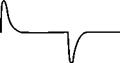
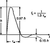
wave, the system reacts in order to restore the resistance (and therefore the voltage) to the initial value (Figure 3.14).

The response time (Figure 3.15) is measured as the time, tw between the beginning of the pulse and a point on the descending curve whose ordinate is 3% of the total pulse. The bandwidth, or cut-off frequency, defined as the frequency at which the amplitude of the output signal is -3dB, can be expressed by

f(-3dB) = 1t1.3Tw

The frequency response can be optimized by adjusting the filter and the gain of the amplifier.

Instability of the system causes the appearance of oscillations in the response of the anemometer bridge that can take two aspects (Figure 3.16):

1. This type of oscillation, due to the difference in inductance between the active and passive arm of the bridge (e. g. the cable connecting the

Determination of the time constant of a CTA

Types of instability

probe to the anemometer is too long), can be removed by adjusting a winding in series with the passive resistance.

2. This oscillation is due both to low bandwidth, in which case it can be removed by increasing the gain, and to an excessive damping of the system, which may be reduced by acting on another winding.

The time constant of the CTA depends on the speed with which the electronic circuit, in response to the attempt to change the temperature of the wire, sends more or less current in the wire; it depends on certain factors such as the thermal properties of the sensor and the fluid, the overheating ratio, the temperature coefficient of resistance, the speed of the fluid, the gain of the amplifier, the resistance of the bridge and the bandwidth of the amplifier. However, it can be said that the time constant of the CTA is linked to that of the CCA by the ratio:

where S = gain of the amplifier. The time constant of the wire is thus reduced a few hundred times, from fractions of ms to some ms. The frequency limit is typically in the order of hundreds of kHz.