Our heavyweight helicopter equal in the world does not have
In Rostov started production of the most load-lifting rotary-wing car The Russian holding «Helicopt[...]

Everything about aircrafts and helicopters. News and events in aviation worldwide. Civil, transportation, military helicopters and airplanes.

Everything about aircrafts and helicopters. News and events in aviation worldwide. Civil, transportation, military helicopters and airplanes.

Everything about aircrafts and helicopters. News and events in aviation worldwide. Civil, transportation, military helicopters and airplanes.

Everything about aircrafts and helicopters. News and events in aviation worldwide. Civil, transportation, military helicopters and airplanes.


In the constant temperature anemometer the influence of the thermal inertia of the sensor is eliminated as the temperature of the wire is
constant whatever the velocity of the stream; the frequency limit of the instrument is therefore essentially determined by the electronic circuit.
1.6.1 Schematic of a CTA
Figure 3.13 illustrates the basic pattern of a CTA: the wire is again in an arm of a Wheatstone bridge opposed to a variable resistor that adjusts the operating resistance, and hence the temperature of the hot wire; the output of the bridge is in this case connected to an amplifier whose output is in turn the supply voltage of the bridge. If the bridge is balanced, there is no potential difference across the diagonal. When the fluid speed increases, the sensor tends to cool and its resistance decreases; an imbalance of the bridge is generated that changes the input signal of the amplifier. The phase of the amplifier is such that the voltage reduction causes an increase of the output signal of the amplifier which increases the current in the sensor and then the temperature until it restores the balance of the bridge.
 |
Schematic of a CTA
If the amplifier has a sufficient gain, it is able to hold the input signal much closer to a balanced bridge, so any change in the resistance of the sensor is immediately corrected by an appropriate variation of the current. The output signal of the system at constant temperature is the output voltage of the amplifier, which, in turn, is the voltage required to ensure the required current through the sensor.
The physical reasoning confirms the trend of E = E(U) of Figure 3.7: if the speed increases ^ heat transfer between the sensor and the fluid increases ^ the sensor tends to cool and its electrical resistance to decrease ^ the amplifier sends more current in the wire to maintain the same resistance ^ the potential difference across the resistor increases.
The overall time constant of the anemometer may be calculated by theoretical considerations; in practical applications, however, the
Response of a CCA to a square wave test at two different speeds of the stream
![]()
 |
![]() V = 0
V = 0
configuration of the probe introduces so many and uncontrollable parameters as to make unreliable the value of tw calculated. On the other hand, to perform even in this case a calibration, one should have either a sample turbulence or make the probe oscillate with the desired frequency in a flow with a constant speed. It is therefore necessary to use indirect methods.
The most accepted method is to send a square wave voltage signal in the wire (in all the commercial anemometers, a square wave generator is provided), which simulates a similar variation of speed, and displays the response of the wire on an oscilloscope at various flow speeds (Figure 3.12). Acting on the circuit components (resistors, overheating ratio, gain of the amplifier), the frequency response of the anemometer can be optimized.
The biggest flaw in the constant current system is the fact that the frequency response of the sensor depends not only on the characteristics of the sensor but also on the characteristics of the fluid stream: the answer depends, as we have seen, both on the heat capacity of the wire and on the coefficient of heat exchange between sensor and environment. In particular, since the sensor response changes with fluid speed, the frequency compensation of the amplifier should be readjusted at every change in the average speed. This is not practical and therefore the anemometer at constant current is used only in cases where the average speed remains constant (steady turbulence).
One of the main reasons for the use of the hot wire anemometer in fluid mechanics is its ability to follow turbulent fluctuations in speed. In the CCA, the key parameter is the heat capacity of the wire which opposes temperature changes; at increasing frequency of speed fluctuations the sensor follows the change of velocity with an increasing delay and the amplitude of the oscillations in output will become smaller compared with that in input. This behavior can be expressed quantitatively by evaluating the frequency response of the CCA.
From Equation (3.2), taking into account Equation (3.7):
– IіRw + (a + b4U)Rw ~ Ra = 0 aRa dt w V > aRa
The differential equation that links the resistance of the wire with time is linear of the first order and it follows that in response to a sudden increase in speed (Figure 3.10) the resistance decreases with the law
Rw = Rw1 – DRw(1 – e-tTw) (3.10)
Response of the resistance of the probe of a CCA to a step increase in the speed of the stream
 Velocity
▲
иг
 |
Ui ——-
where Rw1 is the initial resistance and Rw2 = Rw1 – DRw is the resistance that the wire would reach asymptotically for t = ^. tw is the time constant of the wire
![]()
![]()
![]() (3.11)
(3.11)
that represents the time that resistance takes to reach the value
Rw = Rw1 – DRw (1 – ej = Rw1 – 0.63DR
or, similarly to what has been said for the time constant of a U-tube manometer (cf. Section 1.2.1.2), the time it would take to reach the new equilibrium value if the rate of change were the initial one. As shown in Equation (3.11), the time constant, which is a measure of the change of wire resistance (temperature), increases with the overheating ratio and with the decrease in speed. For the reference probe tw = 0.6 ms.
The time constant can be associated with a cut-off frequency or frequency limit:
which is also the bandwidth of the frequency of the sensor (for the reference probe fc = 300 Hz).
 |
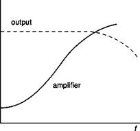 |
Frequency response of sensor, amplifier and CCA
Dryden in 1929 showed that if applying to the sensor a speed variable with a certain frequency, f, the amplitude of the output signal from the sensor is not equal to that which would occur in the steady case but decreases in the ratio (Figure 3.11)
![]() A = 1
A = 1
A = 1 + (//f)2
and that the output signal has a delay of phase with respect to the input signal equal to
![]() Da = tg – (ff)
Da = tg – (ff)
From Equations (3.13) and (3.14) it can be seen that the frequency limit can also be defined as the frequency at which the reduction in amplitude of the power is equal to 1/2 (-3dB) and the phase delay is 45°.
In order to offset the effect of reducing the amplitude of the signal, the amplifier connected with the sensor should have a gain variable with frequency (Figure 3.11) with a reverse law with respect to Equation (3.13); of course also the amplifier has its own inertia for which the best that can be obtained is an extension of the bandwidth of the wire sensor – amplifier system from 300 Hz to a few kHz.
The preceding paragraphs have been devoted mainly to the sensor and its heat exchange with the fluid stream. The sensor must be controlled by an electronic circuit, which is a very important element of the anemometer. It provides a controlled electric current to the sensor and ensures the compensation of frequency. A sensor itself cannot follow speed variations at frequencies above 300 Hz; with electronic compensation this response may be increased to values of the order of kHz.
3.5.1 Schematic of a CCA
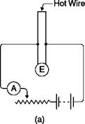
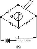
The current in the sensor is maintained essentially constant by using a large resistor in series with the sensor: since the current flowing in the circuit is I = E(R + R„), if R >> Rw, the current will be practically independent of Rw. In practice, a Wheatstone bridge (Figure 3.9 b) is used and the voltage drop across the sensor is measured by the unbalance of the bridge.
A physical point of view confirms the trend of E = E(U) of Figure 3.8: if the speed increases ^ heat transfer between the sensor and the fluid increases ^ the sensor cools down ^ its electrical resistance decreases ^ the potential difference across the resistor decreases (as the current through the sensor is constant). An amplifier picks up this change in voltage and then amplifies the signal to levels useful for recording.
Circuits of constant current anemometers
One of the limitations of the CCA is the fact that if too low an electric current is chosen, at the higher stream speeds the wire is too cold, its temperature tends to air temperature and the sensitivity of the anemometer decreases. Conversely, if too high an electric current is chosen, when the stream speed is too low, the danger of burning the wire exists: this is the case for measures in the boundary layer, where the velocity tends to zero, or in the case of removing the probe from the stream before shutting down the power supply to the wire.
From Equation (3.2) it follows that in steady state the thermal power exchanged between the hot wire and the fluid stream is equal to the electrical power, W, dissipated in the wire by the Joule effect:
![]()
W = I2 Rw = E 2/Rw
where I is the electric current and E is the potential difference across the hot wire. From Equation (3.5), King’s law [1] (Equation 3.6) is obtained, linking the speed, U, to the fourth power of E:
IіRw = R = (a+ b4U){Tw -Ta) King’s law (3.6)
Vw
that taking into account Equation (3.1) becomes:
Equation (3.7) is a relationship between three variables: stream speed, U, electric current, I, and wire resistance, Rw. If the stream speed has to be related to a single variable (current or electrical resistance or potential difference) there are two possible alternatives:
■ holding the electrical resistance (or temperature) of the wire constant and allowing fluctuations of the electrical current with speed (constant temperature anemometer, CTA);
■ holding the electrical current constant: in this way the change in velocity causes a temperature change of the wire and hence of its electrical resistance (constant current anemometer, CCA).
 |
||
Operating at constant resistance, differentiating Equation (3.7) yields:
From Equation (3.8) it follows that (Figure 3.7):
■ the potential difference across the wire increases with increasing speed;
■ the instrument sensitivity decreases with increasing speed.
Operating at constant current the temperature of the wire is free to vary with speed; differentiating Equation (3.7) yields:
1 f3E) =- (Rw – Ra)Ra a(Tw – Ta)
EdUE 2 U + 2 U + abU
|
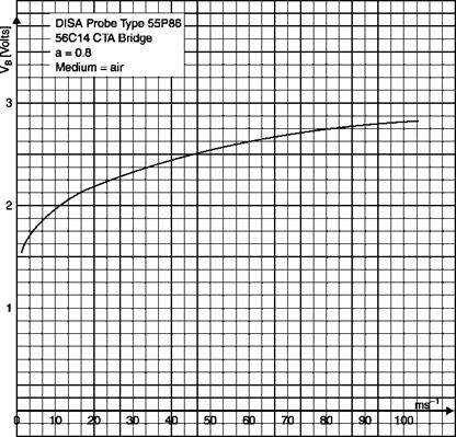
Calibration curve of a CTA
|
From Equation (3.9) it follows that (Figure 3.8):
■ the potential difference across the wire decreases with increasing speed;
■ as for the CTA, the sensitivity decreases with increasing speed.
A final consideration must be made on the effects of free convection that is taken into account by the term “a” in Equations (3.5), (3.6) and (3.7).
The fact that there is a small but finite convective velocity near the wire makes measurement of very low flow speed random. Furthermore, the value of free convection depends on the orientation of the wire (horizontal or vertical), so calibration and measurement have to be made in the same position. In practice, the King’s law, as mentioned earlier, has a lower limit of validity at stream speeds of the order of 5 cm/s.
![]()
 |
Figure 3.8
The wire can be considered as a cylinder of diameter d and length l, with the ratio d/l << 1 (1/240 for the reference probe), placed perpendicular to the direction of the velocity U, which is considered uniform over the entire length of the wire. The thermal power exchanged by convection between the wire at temperature Tw, and the fluid at temperature Ta can be calculated from the equation
Q = hA(Tw – Ta) = nlNudA(Tw – Ta) (3.3)
where h is the film coefficient of heat transfer, A is the lateral surface of the wire, Nud is the Nusselt number referred to the diameter of the wire (Nud = hd/l) and l is the coefficient of thermal conductivity of the fluid. In Equation (3.3) the following assumptions are made:
■ the wire is so thin that the wall temperature is equal to the body temperature
■ flow is incompressible (M << 1), it is indeed assumed that the adiabatic wall temperature and the static temperature, Ta, coincide.
For an indefinite cylinder (l/d ^ ^) the Nusselt number can be expressed as a power function of the Reynolds number (referred to the diameter of the cylinder) and the Prandtl number whose exponents depend on whether the motion is laminar or turbulent. If the motion is laminar (Red < Redcr), which is always true for the hot wire anemometer, as the
"1
diameter of the wire is very small (of the order of mm), it can be considered valid for the empirical equation:
Nud = 0.42Pr0’2 + 0.57Pr0’33 Re/5 (3.4)
after Kramers and van der Hegge Zijnen. For the reference probe immersed in a stream of air at standard temperature and pressure and velocity U = 30 [m/s], Red = 10 and Nud = 2.
In practice, even an indefinite cylinder does not follow Equation (3.4) with sufficient accuracy: the exponent of the Reynolds number is 0.48 at lower speeds and 0.51 at higher speeds. The variation of the exponent is still larger for sensors of finite length such as those used in anemometers. The sensors shaped as cones, wedges or domes show exponents significantly different from 0.5.
Because it is only relevant to have a functional relationship between the Nusselt number and velocity of the stream, as a calibration must be carried out for each probe, one can write:
Nud = a + b^Red
Equation (3.3) becomes:
Q=+ bn/Red)(Tw – Ta) = (a+bJU)) – T (3.5)
where a and b are two constants to be determined by calibration, which include the geometric properties of the wire and the fluid parameters. Since the response of the hot wire anemometer depends on many fluid dynamics parameters, the probe could be used to measure temperature, thermal conductivity, pressure, heat flux in addition to speed. For the same reason, when a single variable is measured, care must be taken to keep constant all the other variables: in particular, when measuring speed, it is important to compensate for any temperature difference between test and calibration or any change in fluid temperature during the test.
Free convection losses are usually negligible, so only forced convection can be taken into account, if:
Red > 2G where fr= ~Ta)
v
where Red is the Reynolds number referred to the diameter, d, of the wire, Gr is the Grashof number, which measures the relative importance of the buoyancy force with respect to the viscous force, b is the coefficient of thermal expansion (= 1/T for perfect gases), g is the acceleration of gravity, n is the kinematic viscosity.
For the reference probe Gr = 5.3 x 10⁻⁶, so the minimum speed for which the free convection can be ignored is 5 cm/s.
Radiation is negligible because the temperature of the wire (up to 300°C) is not too high compared to the ambient temperature.
 |
Effects of conduction to the supports on the distribution of wire temperature
From the energy balance of the wire of the anemometer, heated by the Joule effect and cooled by a fluid stream, we have:
”1
where Cw is the heat capacity of the wire, W is the electrical power supplied to the wire and Q is the thermal power exchanged among the wire and the environment by convection, conduction and radiation.
3.4.1 Conduction to the supports
The supports have a diameter much greater than that of the wire, partly for reasons of robustness and partly to avoid heating up at the passage of electric current; for this reason, the temperature at the end of the wire is very close to the temperature of the fluid, Ta, and thus the heat transfer by conduction along the wire is appreciable (Figure 3.6). Since this effect is quite complicated, especially when there are fluctuations of speed that over time will change the temperature distribution on the wire, it is difficult to make a theoretical evaluation valid in general and it is necessary to calibrate each individual probe.
A wire is stretched between two metal prongs, similar to sewing needles (Figure 3.3). The diameter of the wire is limited by the need to have an adequate electrical resistance, a very rapid response and a high resolution. The diameter normally employed is 5 pm. To increase the size of the
|
Breaking stress x 10-4 (Ncrrr2) |
Maximum temperature (°С) |
Soft- solderable |
Weldable |
Available as Wollaston wire |
Minimum diameter (pm) |
ІЇК1) |
Resistivity at 0°C x 106 fl(cm) |
Thermal conductivity at 0°C (Wcm_1K_1) |
|
|
Tungsten |
20 и – 25 |
300 (oxidizes) melting point 3382 |
No |
Yes if plated |
No |
2.5 4 3.8 |
0.0035 4 0.0047 |
4.9 4 5.5 |
1.9 |
|
Platinum |
2 и – 3.6 |
800 4-1200 melting point 1800 |
Yes |
Yes |
Yes |
1.0 4 1.25 |
0.0030 4 0.0038 |
9.8 4 10 |
0.7 |
|
Platinum- iridium (80/20) |
7 |
750 |
Yes |
Yes |
38 |
0.00085 |
32 |
0.2 |
|
|
Platinum- rhodium (90/10) |
6 |
1400 melting point 1600 |
Yes |
Yes |
Yes |
0.6 |
0.0016 |
9 |
0.4 |
|
Table 3.1 |
|
Sensor materials for hot wire probes |
|
|
||
|
wires in order to make them more manageable during processing and assembly and/or improve the weldability, platinum wire covered with a thick coating of silver (Wollaston wire) or gold-plated tungsten wires are used. After the wire is welded to the supports, the plating is removed with an acid in the zone to be used as a sensor.
The length of the wire is limited by the need to have a good spatial resolution: the sensor simply senses an average speed on its length and the objective is to measure the speed at one point. The length must also be much smaller than the size of the vortices. Plated tungsten wires are used with the minimum length of 1.2 mm (miniature probes). These probes are best used in air flow with turbulence intensity less than 10% and have the highest frequency response; they can be repaired.
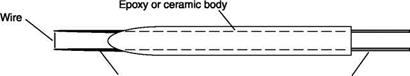
If the wire is too short, aerodynamic interference of the prongs has a not negligible effect and, due to the conduction towards the supports, the temperature of the wire is not uniform. These drawbacks can be alleviated using a longer wire (= 3 mm) of the Wollaston type or plated tungsten and using as a sensor only the central part of it (1 mm) after removing the plating with a chemical attack (Figure 3.4). These probes are used in air streams with intensities of turbulence up to 25% and have a frequency response less than that of miniature probes; they can be repaired.
![]()
 |
Gold-plated sensor
 |
Another type of sensor, called fiber hot film, has replaced the wire in many heavy duty applications (air containing powder, liquid). This type of sensor is made with a quartz fiber on which a film of conductive material covered with quartz is deposited (Figure 3.5). The diameter in this case is the order of 70 pm, the frequency response is lower than that of the wires; they can be repaired.
In addition to the form of wire, hot film sensors can be realized in the most varied shapes: cone or wedge, cylinder, etc. (Figure 3.5). They can be used from low to moderate frequencies of fluctuation of speed; they cannot easily be repaired.
The films are usually made of platinum or nickel, the support is made of Pyrex glass or quartz fiber. If the fluid is a conductive liquid, the sensor must be electrically insulated from the liquid using a thick quartz coating.