Category Aerodynamic measurements

The operation of the hot wire anemometer is based on the fact that the resistance of the wire, Rw, varies with temperature, Tw, according to the linear equation:

Rw = R[1 + a(Tw – T)] (3.1)

where Ra is the resistance at the reference temperature, Ta and а[К-1] is the temperature coefficient of the resistance.

The overheating ratio of the resistor is defined as:

Rw ~ R = a(T – T)

R w a a

The ideal material for the sensor must have a high value of a coupled with a high mechanical strength, be weldable or able to be soft soldered and reduced to wires with a very small diameter, order of pm. Table 3.1 shows the characteristics of the most used materials.

■ The tungsten wires are robust (they are used successfully in supersonic flows) and have a high temperature coefficient of resistance but cannot be used at high temperatures in air because they oxidize easily; they cannot be soldered.

■ Platinum has a good resistance to oxidation, has a good temperature coefficient, but has a low mechanical strength, especially at higher temperatures.

■ The platinum-iridium alloy is to be avoided because it is unstable at high temperatures.

■ The platinum-rhodium alloy is a compromise between tungsten and platinum, with good resistance to oxidation and strength greater than platinum, but has a low temperature coefficient.

To fix ideas about the orders of magnitudes involved, we will refer to a typical sensor consisting of a tungsten wire with length I = 1.2 mm, diameter d = 5 pm, operating temperature Tw = 300°C. Cold resistance is Ra = 3.5 W, the resistance at 300°C is Rw = 7 W, the overheating ratio = 1.

Abstract: This chapter will address the measurement of velocity in unsteady flows in 1D, 2D and 3D fields obtained with hot wire anemometers, from the first analog constant current anemometer in the 1930s to the current solid state digital constant temperature anemometer.

Key words: hot wire, King’s law, turbulence intensity.

3.1 Introduction

As seen in Chapter 2, speed can be obtained from pressure measurements only in almost stationary streams. In turbulent flows it is necessary to use the hot wire anemometer, which has a very high frequency response, or, alternatively, the laser-Doppler anemometer (LDA), the laser-2 focus anemometer (L2F), which are able to infer the intensity of turbulence from a statistical survey of the speeds of many particles carried by the stream.

The sensor of the hot wire anemometer (Figure 3.1) is a metallic wire heated by the Joule effect and cooled by the fluid flow. Because the

Figure 3.1

electrical resistance of the wire changes with temperature, by the changes in the difference of potential at the ends of the wire the corresponding changes in flow velocity can be deduced. Fluctuations in speed can be measured, using appropriate electronics, at a very fine scale at high frequency.

The output signal of the hot wire anemometer is compared in Figure 3.2 with those from the laser-Doppler anemometer and particle image vel – ocimetry (PIV): the advantages of hot-wire anemometer on other systems, in addition to being less costly, are the ease of use, the analog output and a high temporal resolution that allows spectral analysis of the signal.

Note that LDA signals (like those of the L2F) are random: a signal is provided each time a particle passes in the measuring zone, and those of the PIV are cadenced by the frequency with which pairs of consecutive images are taken by a charged-couple device camera.

There are other systems for measuring flow, based on the measurement of the speed of rotation of a small turbine or gear cam. These systems are typically used to know the total mass passed in a given time (gas or fuel meter).

A particular type of mass flowmeter, called a “rotameter,” is widely adopted both in the laboratory and in industrial plants, providing a visual indication of the mass flow rate. The instrument consists of a vertical, transparent and slightly conical tube (Figure 2.39), in which the fluid is introduced from below. A floating body is inserted in the tube and the mass flow rate is read on a scale printed on the wall of the tube: the floating body is in equilibrium at the height where the drag added to the buoyancy force equals its weight. As mass flow rate increases, drag tends to increase and the body moves up to a new larger section where speed, and hence drag, goes back to the previous value.

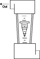Figure 2.39

Often a set of floating bodies of different masses is provided with each rotameter in order to use the same tube for different ranges of mass flow rates. Rotameters are available for a large number of gases at different pressures and for many liquids of industrial interest.

If a large pressure drop can be accepted, a sonic nozzle can be used as a mass flowmeter. In the throat, where the unit Mach number is attained:

so the mass flow rate can be calculated from a measurement of stagnation pressure and stagnation temperature. Even in this case a flow coefficient is used.

Discharge coefficient much closer to 1 can be obtained using a mouthpiece orifice (Figure 2.37) so as to obtain a more regular outflow; the con­struction is obviously more complex. The instrument is more expensive than the plate orifice and is therefore more suitable for a permanent installation. The corresponding discharge coefficients are between 0.96 and 0.99 for 0.3 < A1jA1 < 0.8 and for Reynolds numbers above 104.

2.7.2.1 Venturi tube

The outflow through the plate orifice (to a lesser extent through the mouthpiece) is accompanied by significant losses generated in the vortex produced by the sudden contraction regions, so it is more efficient to use a Venturi tube (Figure 2.38), which is made of a convergent, a constant section tube and a diffuser with a small angle of divergence; the losses of stagnation pressure slightly exceed those that are generated in a tube with a constant section of equal length. The device is rather long and expensive, it is used in permanent installations in power stations and chemical plants.

The static pressure is measured at the entrance of the convergent and in the throat, the discharge coefficient is approximately 0.995.

It must be emphasized here that the quoted values of C are valid only for a well-defined geometry and thus are only a guide for different geometries. In ISO regulations, from where the previous figures are taken,

Figure 2.37

detailed plans of the various types of flowmeters, the rules to be followed when installing and measuring, quality of workmanship and materials to be used are given.

The plate orifice (Figure 2.36) is used in cases where the high pressure drop introduced by the device can be tolerated. The duct is obstructed by a plate with a circular hole, the static pressure is measured at the tube wall immediately upstream and immediately downstream of the orifice.

Figure 2.36

Source: [9]

Since the stream separates from the walls of the duct both upstream and downstream of the orifice, the outflow is strongly swirling and cannot be considered isentropic. Furthermore the stream continues to accelerate downstream of the orifice because of the formation of a vena contracta and thus the static pressure is lower than that corresponding to the assumed uniform flow through the orifice. Of course, due to the strong deviation from the assumption of isentropic motion assumed in the formulation of Equation (2.8), the discharge coefficient, C, is not very close to 1: it varies from 0.6 to 0.8 for area ratios, A2/Ab ranging between 0.2 and 0.75 and for Reynolds numbers, based on the diameter of the orifice and the speed in the orifice, in excess of 5 x 104.

The device is inexpensive, it can easily be adapted to different ranges by simply changing the perforated plate, and it is therefore suitable for laboratory activities.

Measurement of mass flow can be made easier assuming that the motion in the duct is almost one-dimensional (gradual and small variations of area, constant speed in each section, no production of entropy) and incompressible. Between two stations of the tube both the incompressible Bernoulli equation and the conservation of volumetric flow are valid:

UA = U2A2

from which the mass flow in the pipe can be found:

This method of measuring the mass flow rate is used in throttling devices. The advantages of these devices include robustness, reproducibility of the calibration and their insensitivity to the Reynolds number, above certain minimum values, and to the asymmetry and the disturbance caused by duct obstructions and deviations upstream.

Calibration formulas of these devices are always in the form of Equation (2.8) even if the assumptions of validity of that formula are far from being met. Correction factors are introduced:

■ the flow coefficient, C, takes into account that the flow is not truly one-dimensional and isentropic;

■ the expansion factor (coefficient of compressibility), e2, takes into account the variation in density that occurs when the ratio of pressure generated by the throttling device reaches high values.

The formula for throttling devices then becomes:

The mass flow can be determined, by definition, by integrating the distribution of speed in a section of the duct. If the static pressure is constant in each section, it can be measured in a tap on the wall; to know the distribution of velocity it is sufficient to measure the distribution of stagnation pressure.

It is sufficient to introduce a Pitot tube in the duct through the wall and to explore a whole diameter. The exploration should also be repeated along a diameter orthogonal to the first. The method is laborious and unsuitable for routine work but has a high degree of accuracy and should be applied when calibrating a flowmeter. The procedure can be simplified if, as in all practical cases, the flow in the duct is fully developed: under these conditions the average velocity can be determined by measuring the speed on the axis and knowing the relationship existing between the average speed and the speed on the axis (Figure 2.34) which is a function of Reynolds number referred to the diameter of the duct: this ratio is 0.5 in laminar flow and increases to about 0.8 in the turbulent regime.

Ratio between average and maximum speed in a tube as a function of the Reynolds number

Because the Reynolds number is not known a priori, it is necessary to follow an iterative process:

1. Assume a Reynolds number.

2. Read in Figure 2.34 the corresponding ratio between the average speed and the speed on the axis.

3. Measure the speed on the axis.

4. Calculate the average speed.

5. Calculate the Reynolds number.

6. Start again from step 2 until the speed difference between two consecutive iterations is less than the desired approximation.

Since in usual industrial applications the motion is always turbulent, Preston devised an instrument consisting of a tube with a constant section in which four Pitot tubes are placed at intervals of 90° on a circle whose radius is 3/4 of the radius of the pipe; four static taps are made on the wall corresponding to the heads of the Pitot tubes (Figure 2.35). The idea is that at 3/4 of the radius the speed is a constant fraction of the aver­age speed in a wide range of Reynolds numbers and surface roughness.

Figure 2.35

The Preston tube is an ideal instrument to measure the flow in a duct con­nected to a pumping system of limited power because inherent losses are negligible.

To measure the mass flow of a fluid in a duct through measures of pressure, it is necessary that the station in which the measure has to be made be free of vortices and that the axis of the duct be straight (no centrifugal forces and thus no pressure gradient in the direction normal to the axis). The international regulations provide, for any kind of flowmeter, the length of pipe (in diameters) with constant section and straight axis that must separate the measuring station, both upstream and downstream, from valves, elbows, intersections with other tubes and changes in section. For difficult cases, a flow conditioner, consisting of a circular or hexagonal (honeycomb) block of tubes or by one or more perforated plates, should be included in the duct upstream of the measuring station.

Only under these conditions is the static pressure constant in the section and measurable on the wall; for greater safety, usually four holes, placed at 90° in the same section, are placed in communication with each other in a groove around the tube, measuring the resulting pressure gives, somehow, an average of the possibly different pressures prevailing in the four holes.

As with all probes, any reason to disturb the magnitude of the variable to be measured must be avoided; in this case, one must avoid generating a drag in the duct that modifies the flow rate.

In unsteady flow fields it is necessary to use diagnostic instrumentation with a high frequency response. A probe capable of giving instant in­formation on the three components of velocity and static and stagnation pressures in a stream is achieved by including unsteady pressure transducers directly into the body of the probe.

The highest response rate of 5 kHz is obtained with the transducers positioned in the head of the probe (Figure 2.32) with a diameter of

Sectional view of a quick-response probe with transducers embedded in the tip

Sectional view of a five-hole probe with transducers embedded in the shaft

about 13 mm. If smaller heads are needed (about 2 mm in diameter), the transducers must be placed in the shaft (Figure 2.33).