Our heavyweight helicopter equal in the world does not have
In Rostov started production of the most load-lifting rotary-wing car The Russian holding «Helicopt[...]

Everything about aircrafts and helicopters. News and events in aviation worldwide. Civil, transportation, military helicopters and airplanes.

Everything about aircrafts and helicopters. News and events in aviation worldwide. Civil, transportation, military helicopters and airplanes.

Everything about aircrafts and helicopters. News and events in aviation worldwide. Civil, transportation, military helicopters and airplanes.

Everything about aircrafts and helicopters. News and events in aviation worldwide. Civil, transportation, military helicopters and airplanes.


7.2 Trim
The general principle of flight with any aircraft is that the aerodynamic, inertial and gravitational forces and moments about three mutually perpendicular axes are in balance at all times. In helicopter steady flight (non-rotating), the balance of forces determines the orientation of the main rotor in space. The balance of moments about the aircraft centre of gravity (CG) determines the attitude adopted by the airframe and when this balance is achieved, the helicopter is said to be trimmed. To a pilot the trim may be ‘hands on’ or ‘hands off’; in the latter case, in addition to zero net forces and moments on the helicopter the control forces are also zero: these are a function of the internal control mechanism and will not concern us further, apart from a brief reference at the end of this section.
In deriving the performance equation for forward flight in Chapter 5 (Equation 5.70), the longitudinal trim equations were used in their simplest approximate form (Equations 5.66 and 5.67). They involve the assumption that the helicopter parasite drag is independent of fuselage attitude, or alternatively that Equation 5.70 is used with a particular value of DP for a particular attitude, which is determined by solving a moment equation (see Figures 8.2a-c and the accompanying description below). This procedure is adequate for many performance calculations, which explains why the subject of trim was not introduced at that earlier stage. For the most accurate performance calculations, however, a trim analysis programme is needed in which the six equations of force and moment are solved simultaneously, or at least in longitudinal and lateral groups, by iterative procedures such as Stepniewski and Keys (Vol. II) have described.2
Consideration of helicopter moments has not been necessary up to this point in the book. To go further we need to define the functions of the horizontal tailplane and vertical fin and the nature of direct head moment.
1 This chapter makes liberal use of unpublished papers by B. Pitkin, Flight Mechanics Specialist, Westland Helicopters.
2 An illustration of the complexities introduced when a full 6 degree of freedom analysis is taken is the role of the tail rotor. It will be producing a thrust to balance the torque provided by the engine(s) to power the main rotor. This thrust will be a side force which will need to be reacted by a change in the lateral tilt of the main rotor disc. Hence the main and tail rotors have a mutual influence.
Basic Helicopter Aerodynamics, Third Edition. John Seddon and Simon Newman. © 2011 John Wiley & Sons, Ltd. Published 2011 by John Wiley & Sons, Ltd.
|
|
In steady cruise the function of a tailplane is to provide a pitching moment to offset that produced by the fuselage and thereby reduce the net balancing moment which has to be generated by the rotor. The smaller this balancing moment can be, the less is the potential fatigue damage on the rotor. In transient conditions the tailplane pitching moment is stabilizing, as on a fixed-wing aircraft, and offsets the inherent static instability of the fuselage and to some extent that of the main rotor. A fixed tailplane setting is often used, although this is only optimum (fuselage attitude) for one combination of flight condition and CG location.
A central vertical fin is multi-functional: it generates a stabilizing yawing moment and also provides a structural mounting for the tail rotor. The central fin operates in a poor aerodynamic environment, as a consequence of turbulent wakes from the main and tail rotors and blanking by the fuselage, but fin effectiveness can be improved by providing additional fin area near the tips of the horizontal tailplane.[6]
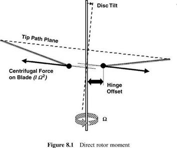
When the flapping hinge axis is offset from the shaft axis (the normal condition for a rotor with three or more blades), the centrifugal force on a blade produces (Figure 8.1) a pitching or rolling moment proportional to disc tilt. Known as direct rotor moment, the effect is large because, although the moment arm is small, the centrifugal force is large compared with the aerodynamic and inertial forces.[7] A hingeless rotor produces a direct moment perhaps four times that of an articulated rotor for the same disc tilt. Analytically this would be expressed by, according to the flexible element, an effective offset four times the typical 3-4% span offset of the articulated hinge.
Looking now at a number of trim situations, in hover with zero wind speed the rotor thrust is vertical in the longitudinal plane, with magnitude equal to the helicopter weight corrected for fuselage downwash. For accelerating away from hover the rotor disc must be inclined forward and the thrust magnitude adjusted so that it is equal to, and directly opposed to, the vector sum of the weight and the inertial force due to acceleration. In steady forward flight the disc is inclined forward and the thrust magnitude is adjusted so that it is equal to, and directly opposed to, the vector sum of the weight and aerodynamic drag.
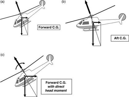
The pitch attitude adopted by the airframe in a given flight condition depends upon a balance of pitching moments about the CG. Illustrating firstly without direct rotor moment or tailplane and airframe moment, the vector sum of aircraft drag (acting through the CG) and weight must lie in the same straight line as the rotor force. This direction being fixed in space, the attitude of the fuselage depends entirely upon the CG position. With reference to Figures 8.2a and b, a forward location results in a more nose-down attitude than an aft location. The effect of a direct rotor moment is illustrated in Figure 8.2c for a forward CG location. Now the rotor thrust and resultant force of drag and weight, again equal in magnitude, are not in direct line but must be parallel, creating a couple which balances the other moments. A similar situation exists in the case of a net moment from the tailplane and airframe. For a given forward CG position, the direct moment makes the fuselage attitude less nose-down than it would otherwise be. Reverse results apply for an aft CG position. At high forward speeds, achieving a balanced state may involve excessive nose-down attitudes unless the tailplane can be made to supply a sufficient restoring moment.
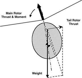
Turning to the balance of lateral forces, in hover the main rotor thrust vector must be inclined slightly sideways to produce a force component balancing the tail rotor thrust. This results in a hovering attitude tilted 2° or 3° to port (Figure 8.3). In sideways flight the tilt is modified to balance sideways drag on the helicopter: the same applies to hovering in a crosswind. In forward flight the option exists, by sideslipping to starboard, to generate a sideforce on
|
Figure 8.2 Fuselage attitude in forward flight: (a) forward CG; (b) aft CG; (c) forward CG with direct head moment |
|
Figure 8.3 Lateral tilt in hover |
the airframe which, at speeds above about 50 knots, will balance the tail rotor thrust and allow a zero-roll attitude to be held.
With the lateral forces balanced in hover, the projection of the resultant of helicopter weight and tail rotor thrust will not generally pass through the main rotor centre, so a rolling couple is exerted which has to be balanced out by a direct rotor moment. This moment depends upon the angle between disc axis and shaft axis and since the first of these has been determined by the force balance, the airframe has to adopt a roll attitude to suit. For the usual situation, in which the line of action of the sideways thrust component is above that of the tail rotor thrust, the correction involves the shaft axis moving closer to the disc axis; that is to say, the helicopter hovers with the fuselage in a small left-roll attitude. Positioning the tail rotor high (close to hub height) minimizes the amount of left-roll angle needed.
Yawing moment balance is provided at all times by selection of the tail rotor thrust, which balances the combined effects of main rotor torque reaction, airframe aerodynamic yawing moment due to sideslip and inertial moments present in manoeuvring.
The achievement of balanced forces and moments for a given flight condition is closely linked with stability. An unstable aircraft theoretically cannot be trimmed, because the slightest disturbance, atmospheric or mechanical, will cause it to diverge from the original condition. A stable aircraft may be difficult to trim because, although the combination of control positions for trim exists, over-sensitivity may make it difficult to introduce any necessary fine adjustments to the aerodynamic control surfaces.
The ability of a helicopter to take off and land vertically and to be able to hover efficiently makes it very suitable to operating from a deck on a ship. However, the location of the deck on the ship, its size and the fact that the ship will be at sea with its motion on the waves and the high winds it will experience make such operation very hazardous. However, the benefits of
shipborne operation have made the development of the naval helicopter a subject of importance. To operate from the ship the helicopter must handle the following factors:
• The deck will be of limited size restricting the aircraft movements.
• The helicopter will have to perform its manoeuvres in high winds.
• The rotor downwash and the airflow over the ship will interact.
• The ship will be moving.
• The visibility of the pilot is very restricted both rearwards and downwards.
These factors affect the method of operation and the design of the aircraft. The touchdown of the landing on the deck is a major point of the landing. It is not subtle and the pilot will plant the helicopter down in a positive fashion. As with all naval aircraft, the vertical velocity at touchdown is usually of the order of double that of a landborne aircraft. This immediately places higher loads on the undercarriage and its mountings on the fuselage. The dynamic characteristics of the undercarriage legs must arrest the downward motion of the helicopter but also provide a very high level of damping as the undercarriage recoils as the axial loads diminish after touchdown. Taking these factors into account, the naval helicopter undercarriage is a sophisticated device which will carry a weight penalty. Having landed, the airframe is usually secured to the deck with a decklock arrangement. These are often carried on the aircraft itself, with the ship providing an attachment such as a steel wire net.
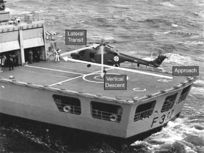
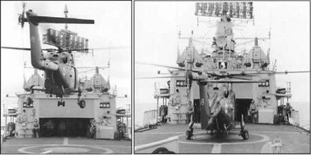
The approach and landing techniques vary, usually between countries. The following is that used by the Royal Navy. One aspect that needs to be emphasized is the lack of pilot’s vision below and behind the aircraft. Additionally, with a two-seat layout in the cockpit, the pilot sits in the right-hand seat when viewed from behind. A typical landing and take-off are illustrated below (see Figure 7.10).
|
|
|
Figure 7.11 A Lynx landing on deck showing the operation of the undercarriage (Courtesy Agusta Westland) |
The approach is made on the port side of the ship with the aircraft coming in on a glide slope of about 3 °. This brings the aircraft to a hover – relative to the ship – at the hangar height and 1.5 to 2 rotor radii off the hull and superstructure. A traverse is then made parallel to the hangar door until the helicopter is hovering above the ship’s centreline. When the ship enters a quiescent state, the aircraft is lowered to the deck, with the aim of a firm touchdown (see Figure 7.10 and Figure 7.11). The undercarriage is designed to arrest the downward motion and also to kill off any tendency to recoil back upwards. If available, a reverse thrust can be selected for the main rotor, pressing the helicopter firmly onto the deck. The decklock is then activated providing a secure mechanical connection to the ship. The main rotor can then be returned to zero thrust. The undercarriage is often fitted with castoring wheels so the helicopter can be manoeuvred on deck using the tail rotor thrust to provide the turning moment.
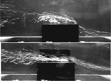
One item of particular importance is the flow conditions surrounding the flight deck. Ship’s flight decks are usually placed at the rear of the ship and with the hangar and hull sides, the flows are typically separating off sharp edges – that is bluff bodies. Figure 7.12 shows two flow types seen in a water tunnel experiment. Both flows are appropriate to wind perpendicular to the ship centreline. The upper image is just a hull and deck where the flow separates off the windward deck edge dividing the flow into a recirculating region above the deck surmounted by a clear airflow directed upwards. The lower image shows the effect of adding a hangar-type structure. There is now a separation line along the upwind hangar door edge. This combines with the original separation line to give a vortex flow which develops from the bottom door corner and covers the entire deck region.
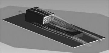
If the flow is coming from the bow, the flow is influenced by the hangar as shown by Figure 7.13 which is a computational fluid dynamics (CFD) calculation.
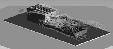
The flow is dominated by the separation off the hangar roof and its eventual reattachment on the deck surface. In reality this reattachment point varies in position with respect to time. It is to this flow state that the helicopter enters as it traverses over the flight deck. The rotor downwash will interact with this flow producing a typical pattern as shown in Figure 7.14.
The flow is completely changed with the rotor downwash providing the main feature. There is now a significant recirculation between the front rotor edge and the hangar door. It is these
|
Figure 7.12 Flow past a hull and a hull-superstructure combination |
|
Figure 7.13 CFD predicted flow over bow – ship only |
|
|
|
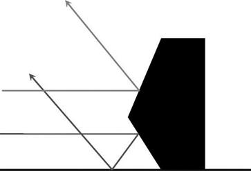
Figure 7.15 Stealth applied to ship profile |
|
|
effects which make shipborne operation so challenging for a helicopter. The separation off the ship’s superstructure will be made more complex with the new breed of warship. In order to introduce stealth the superstructure is significantly changed.
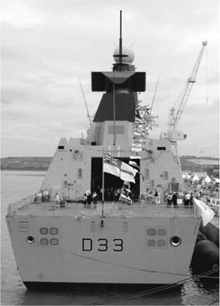
Figure 7.15 shows two incident signals from a radar source and by using inclined surfaces the signals are returned in a specific direction which will minimize any returns to the enemy source. This alignment technique has been used on the more modern fighter aircraft designs. Figure 7.16 shows the flight deck of a Type 45 destroyer, HMS Dauntless, where the inclined faces of the hull and superstructure can be seen.
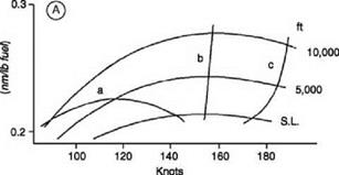
Fixed-wing aircraft operate more economically at high altitude than at low. Aircraft drag is reduced and engine (gas-turbine) efficiency is improved, leading to increases in cruising speed and specific range (distance per unit of fuel consumed). With gas-turbine-powered helicopters, the incentive to realize similar improvements is strong: there are, however, basic differences to be taken into account. On a fixed-wing aircraft, the wing area is determined principally by the stalling condition at ground level; increasing the cruise altitude improves the match between area requirements at stall and cruise. On a helicopter, the blade area is fixed by a cruise speed requirement, while low-speed flight determines the installed power needed. The helicopter rotor is unable to sustain the specified cruising speed at altitudes above the density design altitude, the limitation being that of retreating blade stall. The calculations now to be described are of a purely hypothetical nature, intended to illustrate the kind of changes that could in principle convey a high-altitude flight potential. The altitude chosen for the exercise is 3000 m (10 000 ft), this being near the limit for zero pressurization. We are indebted to R. V. Smith for the work involved.
Imperial units are used as in the previous section. The data case is that of a typical light helicopter, of all-up weight 10 000 lb and having good clean aerodynamic design, though traditional in the sense of featuring neither especially low-drag nor advanced blade design. Power requirements are calculated by the simple methods outlined earlier in the present chapter. Engine fuel flow is related to power output in a manner typical of modern gas-turbine engines. Specific range (nautical miles per pound fuel) is calculated thus:
Specific range(nm/lb) = forward speed((knots)/fuel)flow(lb/hr)
A flight envelope of the kind described in Section 7.7 is assumed: this is primarily a retreating-blade limitation in which the value of W/d (d being the relative density at altitude) decreases from 14000lb at 80 knots to 8000lb at 180 knots.
The results are presented graphically in Figures 7.9A-D.
Specific range is plotted as a function of flight speed for sea level (SL), 5000 ft and 10 000 ft altitude. Intersecting these curves are (a) the flight envelope limit, (b) the locus of best-range speeds and (c) the power limitation curve. We see that in case A, which is for the data helicopter, the flight envelope restricts the maximum specific range to 0.219 nm/lb, this
 |
|
Table 7.3 Comparison of configuration performance
|
occurring at 5000 ft and low speed (only 114 knots). So far as available power is concerned, it would be possible to realize the best-range speeds up to 10000 ft and beyond.
Case B examines the effect of a substantial reduction in parasite drag. Using a less ambitious target than that envisaged in Section 7.9, a parasite drag two-thirds that of the data aircraft is assumed. At best-range speed a large increase in specific range at all altitudes is possible but, as before, the restriction imposed by the flight envelope is severe, allowing an increase to only
0. 231 nm/lb, again at approximately 5000 ft and low speed (120 knots). It is clear that the full benefit of drag reduction cannot be realized without a considerable increase in rotor thrust capability. A comparison of cruising speeds emphasizes the deficiency: without the flight- envelope limitation the best-range speeds would be usable, that is at all heights a little above 150 knots for the data aircraft and 20 knots higher for the low-drag version.
The increase in thrust capability required by the low-drag aircraft to raise the flight envelope limit to the level of best-range speed at 10000 ft is approximately 70%. Case C shows the performance of the low-drag aircraft supposing the increase to be obtained from the same percentage increase in blade area. Penalties of weight increase and profile power increase are allowed for, assumed to be in proportion to the area change. The best-range speed is now attainable up to over 9000 ft, while at 10 000 ft the specific range is virtually the same as at best – range speed, that is 0.267 nm/lb at 170 knots; this represents a 22% increase in specific range over the data aircraft, attained at 60 knots higher cruising speed.
For a final comparison, case D shows the effect of obtaining the required thrust increase by combination of a much smaller increase in blade area (24.5%) with conversion to an advanced rotor design, using an optimum distribution of cambered blade sections and the Westland advanced tip. The penalties in weight and profile power are thereby reduced considerably. The result is a further increase in specific range, to 0.293 nm/lb or 34% above that of the data aircraft, attained at the same cruising speed as in case C.
The changes are seen to further advantage by calculating also the maximum range achievable. This has been done in alternative ways, assuming that the weightpenalty reduces (1) the fuel load or (2) the payload. On the first supposition, the weight penalty of case C results in a range reduction but with case D the gain more than compensates for the smaller weight penalty.
The characteristics of the various configurations are summarized in Table 7.3.
The ideas in this section come mainly from M. V. Lowson [4]. It is of interest to consider, at least in a hypothetical manner, the lowest level of cruising power that might be envisaged for a really low-drag helicopter of the future, by comparison with levels typically achieved in current design. The demand for fuel-efficient operation is likely to increase with time, as more rangeflying movements are undertaken, whether in an industrial or a passenger-carrying context. Any increase in fuel costs will narrow the operating cost differential between helicopters (currently dominated by maintenance costs) and fixed-wing aircraft, and the possibility of the helicopter achieving comparability is an intriguing one.
Reference to Figure 7.3 shows that at high forward speed, while all the power components need to be considered, the concept of a really low-drag (RLD) helicopter stands or falls on the possibility of a major reduction in parasite drag being achieved. This is not a priori an impossible task, since current helicopters have from four to six times the parasite drag of an aerodynamically clean fixed-wing aircraft. For the present exercise let us take as the data case a 4500 kg (10 000 lb) helicopter, the parasite drag of which, in terms of equivalent flat plate area, is broken down in Table 7.1. All calculations were made in imperial units and for simplicity
|
Table 7.1 Comparison of datum and target aircraft drag data
|
these are used in the presentation. The total, 14.05 ft2, is somewhat higher than the best values currently achievable but is closely in line with the value of 19.1 ft2 for an 18 000 lb helicopter used by Stepniewski and Keys (Vol. II) for their typical case.
In setting target values for the RLD helicopter, as given in Table 7.1, the arguments used are as follows. Minimum fuselage drag, inferred from standard texts such as Hoerner [2] and Goldstein [5], would be based on a frontal area drag coefficient of 0.05. This corresponds to 2 ft2 flat plate area in our case, which is not strictly the lowest possible because helicopters traditionally have spacious cabins with higher frontal areas, weight for weight, than fixed-wing aircraft. A target value of 2.3 ft2 is therefore entirely reasonable and might even be bettered. The reductions in nacelle and tail unit drags may be expected to come in time and with special effort. A large reduction in rotor head drag is targeted but the figure suggested corresponds to a frontal area drag coefficient about double that of a smooth ellipsoidal body, so while much work would be involved in reshaping and fairing the head, the target seems not impossible of attainment. Landing-gear drag is assumed to be eliminated by retraction or other means. In the miscellaneous item of the data helicopter, a substantial portion is engine-cooling loss, on which much research could be done. Tail rotor head drag can presumably be reduced in much the same proportion as that of the main rotor head. Roughness and protuberance losses will of course have to be minimized.
In total the improvement envisaged is a 64% reduction in parasite drag. Achievement of this target would leave the helicopter still somewhat inferior to an equivalent clean fixed – wing aircraft.
Such a major reduction in parasite drag will leave the profile power as the largest component of RLD power at cruise. The best prospect for reducing blade profile drag below current levels probably lies in following the lead given by fixed-wing technology in the development of supercritical aerofoil sections. Using such sections in the tip region postpones the compressibility drag rise to higher Mach number: thus a higher tip speed can be used which, by Equation 6.45, reduces the blade area required and thereby the profile drag. Advances have already been made in this direction, but whereas in the rotor design discussed in Chapter 6 a tip Mach number 0.88 was assumed, in fixed-wing research drag-rise Mach numbers as high as
0. 95 were described by Haines [6]. Making up this kind of deficiency would reduce blade profile drag by about 15%. If it is supposed that in addition advances will be made in the use of thinner sections, a target of 20% lower profile power for the RLD helicopter seems reasonable.
Reduction in induced power will involve the use of rotors of larger diameter and lower disc loading than in current practice. Developments in blade materials and construction techniques will be needed for the higher aspect ratios involved. These can be expected, as can also the relaxation of some operational requirements framed in a military context, for example that of take-off in a high wind from a ship. A 10% reduction of induced power at cruise is therefore anticipated. The same proportion is assumed for the small residual power requirement of the miscellaneous items.
Table 7.2 shows the make-up of cruise power at 160 knots from Figure 7.3, representing the data aircraft, and compares this with the values for the RLD helicopter according to the foregoing analysis.
The overall reduction for the RLD helicopter is 41% of the power requirement of the data aircraft. An improvement of this magnitude would put the RLD helicopter into a competitive position with certain types of small, fixed-wing, propeller-driven business aircraft for low- altitude operation. Qualitatively it may be said that the RLD helicopter has a slightly higher parasite drag than the fixed-wing aircraft, about the same profile drag or slightly less (since the fixed-wing aircraft normally carries a greater wing area than is needed for cruise, while the
|
Table 7.2 Comparison of datum and target aircraft power data
|
helicopter blade area can be made to suit, provided that adverse Mach effects are avoided) and a lower induced drag if the rotor diameter is greater than the fixed-wing span. The helicopter, however, has no ready answer to the ability of the fixed-wing aircraft to reduce drag by flying at high altitude. Equally of course, the fixed-wing aircraft cannot match the low-speed and hover capability of the helicopter.
In the context of advanced rotor blade design as discussed in Chapter 6, and as an example of realized performance, it is of interest to record the capture of the world speed record for
helicopters by a Westland Lynx aircraft in August 1986. The incentive to make the attempt was provided by the results of a programme of test flying on the Lynx fitted with an experimental set of blades in which lift-enhancing aerofoil sections of the RAE ‘96’ Series (Section 6.2) were used throughout the length of the blade, together with the Westland tip design (Section 6.3) combining a sweepback benefit on local Mach number with delaying the tip stall. The tests showed the flight envelope to be improved by the equivalent of 35-40% increase in blade area and made it clear that level flight speeds beyond the existing record were achievable.
Different aerofoil sections were used for the inboard, mid-span and tip parts of the blade, chosen in relation to the local speed conditions and lift requirements. The section used for the tip was thinner than the other two. The blade was built in glass fibre with a single spar, special construction methods being employed.
The aircraft was a standard Lynx (Utility version) with a skid undercarriage, in which protuberance drag had been reduced to a minimum and an attempt had been made to reduce rotor head drag by fairings. The engine power was enhanced by water-methanol injection. The purpose of these measures was to ensure that, given a large alleviation in the flight envelope, the aircraft would not then be power limited unnecessarily.
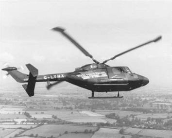
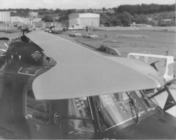
For the record attempt, the course of 15 km was flown at 150 m above ground over the Somerset Levels, this being well within the altitude band officially required. The mean speed of two runs in opposite directions was 400.87 km/h (216 knots), exceeding the previous record by 33 km/h. The aircraft also had an extraordinarily good rate of climb near the bucket speed (80-100 knots), this being well over 20 m/s (4000 ft/min) – exceeding the capacity of the indicator instrument – and generally exhibited excellent flying characteristics. Figure 7.7 shows a photograph of the aircraft in flight and Figure 7.8 presents a spectacular view of the rotor blade.
|
|
|
Figure 7.8 BERP rotor blade on world speed record helicopter (G-LYNX) (Courtesy Agusta Westland) |
The ability to deploy computer methods in performance calculation has been a major factor in the rapid development of helicopter technology since the Second World War. Results may often not be greatly different from those derived from the simple analytical formulae, but the fact that the feasibility of calculation is not dependent upon making a large number of challengeable assumptions is important in pinning down a design, making comparisons with flight tests or meeting guarantees. So it is that commercial organizations and research centres are equipped nowadays with computer programs for use in all the principal phases of performance calculation – hover characteristics, trim analysis, forward flight performance, rotor thrust limits and so on.
It may be noted en passant that performance calculation is generally not the primary factor determining the need for numerical methods. The stressing of rotor blades makes a greater demand for complexity in calculation. Another highly important factor is the need for quantification of handling characteristics, as for example to determine the behaviour of a helicopter flying in an adverse aerodynamic environment.
Within the realm of performance prediction are contained many sub-items, not individually dominant but requiring detailed assessment if maximum accuracy is to be achieved. One such sub-item is parasite drag, in toto an extensive subject, as with fixed-wing aircraft, about which not merely a whole chapter but a whole book could be written. For computation purposes the total drag needs to be broken down into manageable groupings, among which are streamlined and non-streamlined components, fuselage angle of attack, surface roughness, leakage and cooling-air loss. Maximum advantage must be taken of the review literature, as compiled by Hoerner [2], Keys and Wiesner [3] and others, and of background information on projects similar to the one in hand.
Once a best estimate of parasite drag has been made, the accuracy problem in power calculation devolves upon the induced and profile items, as Equation 7.12 shows, together with the additional sub-items of tail rotor power, transmission loss and power to auxiliaries. Improving the estimation of induced and profile power comes down to the ability to use a realistic distribution of induced velocity over the disc area and the most accurate blade section lift and drag characteristics, including dynamic effects. This information has to be provided separately; the problem in the rotor is then to ascertain the angles of attack and Mach numbers of all blade sections, these varying from root to tip and round the azimuth as the blade rotates. That is basically what the focal computer programs do. Iterative calculations are normally required among the basic equations of thrust, collective and cyclic pitch and the flapping angles. A primary difficulty with helicopter rotor analysis is that one cannot solve a subset of the rotor equations – one has to address the interactions all together. Starting with, say, values of thrust and the flapping coefficients, corresponding values of the pitch angle, collective and cyclic, can be calculated; the information then allows the blade angles and local Mach numbers to be determined, from which the lift forces can be integrated into overall thrust for comparison with the value initially assumed. When the iterations have converged, the required output data – power requirement, thrust limits, and so on – can be ascertained.
These brief notes provide an initial examination. Going more deeply into the subject would immerse one immediately into more detail, so a calculation strategy using spreadsheets is provided in the Appendix. In addition, an excellent and thorough exposition of the total process of performance prediction is available in Stepniewski and Keys (Vol. II), to which the reader who wishes to come to grips with the whole computational complex is also referred.
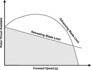
The envelope of rotor thrust limits is the combination of operation on the blades at the stall boundary both at high angle of incidence and with the compressibility effects at high Mach number. Usually the restrictions occur within the limits of available power. The nature of the envelope is sketched in Figure 7.6.
|
Figure 7.6 Nature of rotor thrust limits |
In hover, conditions are uniform around the azimuth and blade stall sets a limit to the thrust available. As forward speed increases, maximum thrust on the retreating blade falls because of the drop in dynamic pressure (despite some increase in maximum lift coefficient with decreasing resultant Mach number) and this limits the thrust achievable throughout the forward speed range. By the converse effect, maximum thrust possible on the advancing side increases but is unrealizable because of the retreating-blade restriction. However, at higher speeds, as the advancing-tip Mach number approaches 1.0, its lift becomes restricted by shock- induced flow separation, leading to drag rise or pitching moment divergence, which eventually limits the maximum speed achievable. Thus the envelope comprises a limit on thrust from retreating-blade stall and a limit on forward speed from advancing-blade Mach effects. Without the advancing-blade problem, the retreating-blade stall would itself eventually set a maximum to the forward speed, as the figure-of-eight diagrams in Figure 6.1 show.
Calculation of the limits envelope is best done by computer, allowing the inclusion of sophisticated factors, natural choices among which are a non-uniform induced-velocity distribution, a compressibility factor on lift slope (usually 1/8 where 8 = (1— M2)l=2, M being the blade section Mach number) and a representation of blade dynamic stall characteristics.
An example of the way in which the limits envelope can dominate performance issues is given later in Section 7.10.
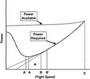
The maximum speed attainable in level flight is likely to be limited by the envelope of retreating-blade stall and advancing-blade drag rise (Section 7.7). If and when power limited, it is defined by the intersection of the curves of shaft power required and shaft power available, (C) in Figure 7.5. In the diagram the power available has been assumed to be greater than that required for hover (out of ground effect) and, typically, to be nearly constant with speed, gaining a little at high speed from the effect of ram pressure in the engine intakes.
Approaching maximum speed, the power requirement curve is rising rapidly owing to the V3 variation of parasite power. For a rough approximation one might suppose the sum of the other components, induced drag, profile drag and miscellaneous additional drag, to be constant and equal to, say, half the total. Then at maximum speed, writing PPARA for the parasite power, we have:
Pav = 2Ppara = pVMax/ (7.14)
whence:
For a helicopter having 1000 kW available power, with a flat plate drag area of 1 m2, the top speed at sea-level density would by this formula be 93.4 m/s (181 knots).
Increasing density altitude reduces the power available and may either increase or decrease the power required. Generally the reduction of available power dominates and VMAX decreases. Increasing weight increases the power required (through the induced power Pj) without changing the power available, so again VMAX is reduced.
The bucket shape of the level flight power curve allows the ready definition of speeds for optimum efficiency and safety for a number of flight operations. These are illustrated in Figure 7.5. The minimum power speed (point A) allows the minimum rate of descent in autorotation. It is also, as discussed in the previous section, the speed for maximum rate of
|
|
climb, subject to a correction to lower speed (A0) if the parasite drag is increased appreciably by climbing. Subject to a further qualification, point A also defines the speed for maximum endurance or loiter time. Strictly the endurance relates directly to the rate of fuel usage, the curve of which, while closely similar to, is not an exact copy of the shaft power curve, owing to internal fuel consumption within the engine: the approximation is normally close enough to be acceptable.
Maximum glide distance in autorotative descent is achieved at speed B, defined by a tangent to the power curve from the origin. Here the ratio of power to speed is a minimum: the condition corresponds to that of gliding a fixed-wing aircraft at its maximum lift-to-drag ratio. Point B is also the speed for maximum range, subject to the fuel-flow qualification stated above. This is for the range in zero wind: in a headwind the best-range speed is at B0, obtained by striking the tangent from a point on the speed axis corresponding to the wind strength. Obviously, for a tailwind the tangent is taken from a point on the negative speed axis, leading to a lower best – range speed than B. This is discussed in more detail in the Appendix.
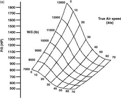
As a first approximation let us assume that for climbing flight the profile power and parasite power remain the same as in level flight and only the induced power has to be reassessed.
|
|
|
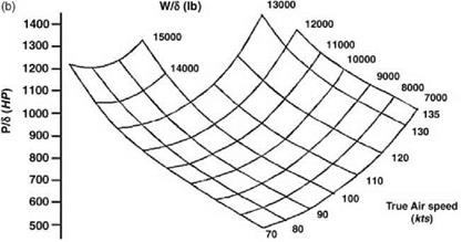
Figure 7.4 (a) Power carpet for rapid calculation (low speed). (b) Power carpet for rapid calculation (high speed) |
The forced downflow alleviates the Vi term but the climb work term, TVC, must be added. In coefficient form the full power equation is now:
1 1 f
Cp = kiliCT + Cd0S [1 + km2] + rm3 + IcCt (7-12)
8 2 A
The usual condition for calculating climb performance is that of minimum power forward speed. In this flight regime, Vi is small compared with V, its variation from level flight to climb
can be neglected and the incremental power DP required for climb is simply TVC. Thus the rate of climb is given by:
|
|
The result is a useful approximation but requires qualification on the grounds that since climbing increases the effective nose-down attitude of the fuselage, the parasite drag may be somewhat higher than in level flight. Also, because the main rotor torque is increased in climb – Equation 7.12- an increase in tail rotor power is needed to balance it. Some of the incremental power available is absorbed in overcoming these increases and hence the climb rate potential is reduced, perhaps by as much as 30%. A further effect is that the increase in drag moves the best climb speed to a somewhat lower value than the level flight minimum power speed.
For a given aircraft weight, the incremental power available for climb decreases with increasing altitude, mainly because of a decrease in the engine performance characteristics. When the incremental power runs out at best climb speed the aircraft has reached its absolute ceiling at that weight. In practice, as Equation 7.13 shows, the absolute ceiling can only be approached asymptotically and it is normal to define instead a service ceiling as the height at which the rate of climb has dropped to a stated low value, usually about 0.5 m/s (100 ft/min). Increasing the weight increases the power required at all forward speeds and thereby lowers the ceiling.