Category BASIC HELICOPTER AERODYNAMICS

As previously discussed, the flapping behaviour of a rotor blade is governed principally by the balance between the aerodynamic lift and the centrifugal force moments about the flapping hinge. These are both dependent on the square of the rotor speed and so, under atmospherically still conditions, the balance is preserved at any rotor speed. However, when operating in high wind conditions, such as on a ship, the balance can be upset. During any helicopter sortie, the rotor must be spun up to speed from rest (engagement) and slowed to a halt (disengagement). At the low-speed ends of these sequences the centrifugal moment is of a small magnitude but the aerodynamic moment can be enhanced by the adverse wind conditions and the blade can experience excessive flapping angles. This is known as blade sailing or, because of its potential to inflict damage to the upper tail boom, tunnel strike.

4.1.1 Lagging Motion

As already described, the helicopter rotor must attain a trimmed condition in forward flight. The disparity between the advancing and retreating sides of the disc is handled by the inclusion of flapping hinges on the rotor hub. Flapping motion introduces a phenomenon associated with a rotating system – that is, the rotor hub. This is the Coriolis acceleration.

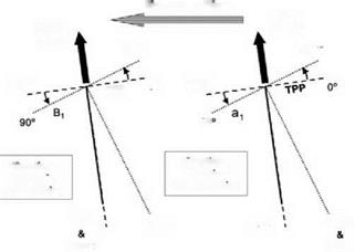
The performance of the rotor blade depends upon its angle of incidence to the TPP. A given blade incidence can be obtained with different combinations of flapping and feathering. Consider the two situations illustrated in Figure 4.20.

These are views from the left side with the helicopter in forward flight in the direction shown. In situation 1 the shaft axis coincides with the TPA; there is therefore no flapping but the necessary blade incidences are obtained from feathering according to Equation 4.9. Blade attitudes at the four quarter points of a rotation are as indicated in the diagram. In situation 2 the shaft axis coincides with the NFA. By definition this means that feathering is zero; the blade angles, however, are obtained from flapping according to Equation 4.5. It is seen that if the feathering and flapping coefficients B1 and a1 are equal, the blade attitudes to the TPP are identical around the azimuth in the two situations. The blade perceives a change in nose-down feathering, via the swashplate, as being equivalent to the same angle change in nose-up flapping.

A pilot uses this equivalence in flying the helicopter, for example to trim the vehicle for different positions of the centre of gravity (CG). The rotor thrust, in direction and magnitude, depends upon the inclination of the TPP in space and the incidence of the blades relative to it. The same blade incidence can be achieved, as we have seen, either with nose-up flapping or with the same degree of nose-down feathering, or of course with a combination of the two. By adjusting the relationship, using the cyclic control stick, the pilot is able to

Direction of Flight

Thrust

Thrust

270°

0° 180°

Shaft

Figure 4.20 Equivalence of flapping and feathering. (Blade chordwise attitudes are shown in the plane of the diagram for azimuth angles of 90° and 270° and normal to the diagram for 0° and 180°)

compensate for different nose-up or nose-down moments in the helicopter, arising from different CG positions. The angle of the shaft axis to the vertical, hence the attitude of the helicopter in space, varies with the CG position but the TPP remains at a constant inclination to the direction of flight.

Control of the helicopter in flight involves changing the magnitude of rotor thrust or its line of action or both. Almost the whole of the control task falls to the lot of the main rotor and it is on this that we concentrate. (The main rotor controls heave, surge/pitch, sway/roll, while yaw is controlled by a tail rotor or similar installation.) A change in line of action of the thrust would, in principle, be obtained by tilting the rotor shaft, or at least the hub, relative to the fuselage. Since the rotor is engine driven (unlike that of an autogyro), tilting the shaft is impracticable. It was attempted with the Cierva W9 as described in Chapter 1. Tilting the hub is possible with some designs but the large mechanical forces required restrict this method to very small helicopters. Use of the feathering mechanism, however, by which the pitch angle of the blades is varied, either collectively or cyclically, effectively transfers to the aerodynamic forces the work involved in changing the magnitude and direction of the rotor thrust.

Blade feathering, or pitch change, could be achieved in various ways. Thus Saunders [1] lists the use of aerodynamic servo tabs, auxiliary rotors, fluidically controlled jet flaps, or pitch links from a control gyro as possible methods.

The widely adopted method, however, is through a swashplate system, illustrated in Figure 4.14 (NFP is the No-Feathering Plane which is discussed later in the chapter.), which shows the operation with collective pitch, while Figure 4.15 shows the operation with cyclic pitch. Carried on the rotor shaft, this embodies two parallel star-shaped plates, the lower of which does not rotate (swashplate or non-rotating star) with the shaft but can be tilted in any direction by operation of the pilot’s cyclic control column and raised or lowered by means of the collective lever. The upper plate (spider or rotating star) is connected by control rods to the feathering hinge mechanisms of the blades and rotates with the shaft, while being constrained to remain parallel to the lower plate through a common bearing assembly. Raising the collective lever thus increases the pitch angle of the blades by the same amount all round (Figure 4.14), while tilting

Advancing

Blade

Figure 4.15 Principles of the swashplate system (cyclic pitch)

the cyclic column applies a tilt to the plates and thence a cyclic pitch change to the blades (Figure 4.15), these being constrained to remain at constant pitch relative to the upper plate.

Figure 4.16 shows a typical control layout of a helicopter cockpit. It is an early design and is very simple. The aircraft is a Saunders Roe Skeeter, and while dual controls are provided, the pilot normally sits in the right-hand seat. More modern helicopters look more complicated with other system controls placed on the collective lever or cyclic stick, but are the same in essence.

An increase of collective pitch at constant engine speed increases the rotor thrust (short of stalling the blades), as for take-off and vertical control generally. A cyclic pitch change alters the line of action of the thrust, since the TPP of the blades, to which the thrust is effectively perpendicular, tilts in the direction of the swashplate angle.

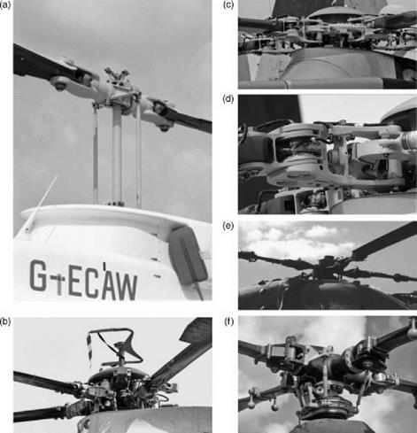
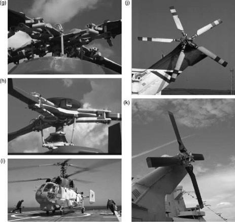
Rotor head designs vary considerably in detail as shown in Figures 4.17a-k. Figure 4.17a shows the simplest rotor head arrangement, namely the two-bladed teetering type. Figure 4.17b

shows a typical articulated rotor as used on the Sikorsky S61N. Figure 4.17c also shows a modern rotor of the fully articulated type. It is of an Agusta Westland Merlin and shows its location on top of the fuselage. Items discernible in the figure include the flap and lag elastomeric hinges, the feathering housing, the lag damper, the pitch control rods and the dual load path blade attachment.

Figure 4.17d shows a close-up view of a Merlin rotor head blade attachment and the blade restraint mechanism of the droop and anti-flap stops can be seen as a horizontal pin fitting into a slot. The main rotor blade folding mechanism is also shown. A good impression is gained of the mechanical complexity of this rotor head installation.

Figure 4.17e shows the semi-rigid rotor of the Westland WG30 (with vibration absorber fitted).

Figure 4.17f shows theMBB Bo 105 rotor head with pendulum vibration absorbers fitted to each blade attachment. The modern strap construction of the Bell 412 is shown in Figure 4.17g, which also has pendulum vibration absorbers installed.

Figure 4.17h shows the ‘Starflex’ rotor of the Eurocopter Ecureuil.

Figure 4.17i shows the complexity of a coaxial rotor system. The aircraft is the Kamov Helix and has two contra-rotating three-bladed rotors on the same shaft.

In comparison, the tail rotor of a Sikorsky S61NM is shown in Figure 4.17j while that of a Merlin is shown in Figure 4.17k.

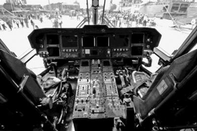
Figure 4.18 is an interior view of the cockpit of a modern helicopter (dual controls).

The collective pitch lever is down at seat level on the pilot’s left (right-hand seat); the cyclic control stick is directly in front between the knees. The foot pedals control the collective pitch of the tail rotor (normally its only control), the purpose of which is to balance the torque of the main rotor, or when required to change the heading of the aircraft.

Cyclic pitch on the main rotor implies a blade angle changing with azimuth, relative to the SNP. The once-per-cycle periodicity means that the pitch angle can be described mathemati­cally by a negative Fourier series, in like manner to that used for the flapping angle.

We write:

У = $o —A1 cos C-B sin ф—А2 cos 2ф—Б2 sin 2C •••

The physical design of a swashplate system only permits once per revolution changes in the pitch angle so only the constant and first harmonic terms are normally required:

в = в0— A1 cos ф—В1 sin C (4-9)

• The constant term в0 represents the collective pitch.

• The terms in C represent the cyclic pitch:

– The factor A1, which applies maximum pitch when the blades are at 0° and 180°, is referred to as the lateral cyclic coefficient because the rotor response, phased 90°, produces a control effect in the lateral sense.

– The factor B1 is the longitudinal cyclic coefficient.

The value of pitch angle would be different if a different reference plane were used. In any flight condition, there is always one plane relative to which the blade pitch remains constant with azimuth. This, by definition, is the plane of the swashplate, which is therefore known as the control plane or, referring to the elimination of cyclic pitch variation, the no-feathering plane

(NFP). NFP, though not fixed in the aircraft, is a useful adjustable datum for the measurement of aerodynamic characteristics considered in the next chapter.

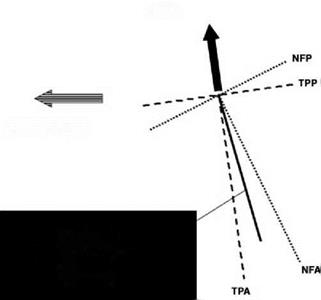
In some contexts it is useful to refer to the axes TPA and NFA, perpendicular to the TPP and NFP, rather than to the planes themselves. Generally in forward flight these two axes and also the shaft axis will be away from the vertical (i. e. the normal to the flight path). Figure 4.19

Rotor

Thrust

Direction of Flight

Shaft Axis
(determines attitude
of helicopter
fuselage)

shows a common arrangement. The thrust line being inclined in the direction of flight, the TPP normal to it is tilted down at the nose relative to the horizontal (the flight direction). The TPA, being also the thrust line, is away from the vertical as shown. The shaft axis is tilted further from the vertical, the angle with the TPA being the tilt-back angle of the flapping motion. The inclination of the shaft axis to the NFA depends upon the degree of feathering in the helicopter motion.

To examine the flapping motion more fully we assume, unless otherwise stated, that the flapping hinge is on the axis of rotation. This simplifies the considerations without hiding anything of significance.

Referring to Figure 4.12, the flapping takes place under conditions of dynamic equilibrium, about the hinge, between the aerodynamic lift (the external forcing function), the centrifugal
force (the ‘spring’ or restraining force) and the blade inertia. (The aerodynamic lift varies as the blade flapping responds in a manner which acts as a damper.) In other words, the once-per-cycle oscillatory motion is that of a dynamic system in resonance. The flapping moment equation is seen to be:

(4.3)

We shall return to this equation later.

The centrifugal force supplies, by far, the largest force acting on the blade and it creates the moment which provides an essential stability to the flapping motion – essentially it acts as a spring. The degree of stability is highest in the hover condition (where the flapping angle is constant) and decreases as the advance ratio increases. Bramwell’s consideration of the flapping equation (p. 153ff.) leads in effect to the conclusion that the motion is dynamically stable for all realistic values of ц.

For normal forward flight, the maximum flapping velocities (b) occur where the resultant air velocity is at its highest and lowest, that is at 90° and 270° azimuth. Maximum displacements occur 90° later, that is at 180° (upwards) and 0° (downwards). As will be seen, the flapping has a natural frequency very close to that of the rotor speed. It is therefore close to a resonant condition which will give a phase delay of near 90° (exactly 90° for a zero hinge offset). While it is near resonance, the aerodynamics provides the damping to keep the responses under control. As already outlined, these displacements mean that the plane of rotation of the blade tips, the tip-path plane (TPP), is tilted backwards relative to the plane normal to the rotor shaft, the shaft normal plane (SNP).

In hover, the blades cone upwards at a constant angle to the SNP, known as the coning angle, usually denoted by a0. Its existence has an additional effect on the orientation of the TPP during rotation in forward flight.

Figure 4.13 shows that, because of the coning angle, the flight velocity Vhas a lift-increasing effect on a blade at 180° (the forward blade) and a lift-decreasing effect on a blade at 0° (the rearward blade). This asymmetry in lift is, we see, at 90° to the side-to-side asymmetry discussed earlier: its effect is to tilt the TPP laterally and since the point of lowest tilt follows 90° behind the point of lowest lift, the TPP is tilted downwards on the advancing side which, with, a rotor rotating anticlockwise from above, is to the right. The coning and disc tilt angles are normally no more than a few degrees.

Since in any steady state of the rotor the flapping motion is periodic, the flapping angle can be expressed in the form of a Fourier series:

b = a0—aj cos C—bi sin C—a2 cos 2ф—Ь2 sin 2C… (4-4)

Textbooks vary both in the symbols used and in the sign convention adopted. The use of negative signs for the harmonic terms is a throwback to the emergence of the autogyro where a rearward disc tilt was the norm, and where the coefficients aj and Ь have positive values. For most purposes the series can be limited to the constant and first harmonic terms – which represent the coned rotor and the disc tilt – thus:

b = a0—a cos C—Ьі sin C

This form will be used in the aerodynamic analysis of the next chapter. For the moment we note that:

• a0 is the coning angle;

• a1 is the angle of backward disc tilt;

• b1 is the angle of sideways disc tilt (advancing side down).

The inclusion of second or higher harmonic terms would represent perturbations about the TPP (in-plane weaving) but any such is of secondary importance only.

Timewise derivatives of b will be needed in the later analysis: using the fact that the rotational speed Q is d^/dt, these are:

The transformation to b as a function of C, the blade azimuth, makes the solutions more informative and therefore useful. It also has the benefit of causing many scaling terms to cancel out.

4.1 The Edgewise Rotor

In level forward flight the rotor is essentially edgewise on to the air stream, a basically unnatural state for propeller functioning. This is shown in Figure 4.1. Practical complications which arise from this have been resolved by the introduction of mechanical devices, the functioning of which in turn adds to the complexity of the aerodynamics.

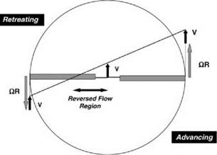
Figure 4.2 pictures the rotor disc as seen from above. Blade rotation is in an anticlockwise sense with rotational speed O. Forward flight velocity is V and the ratio V/OR, R being the blade radius, is known as the advance ratio and given the symbol p. It has a value normally within the range 0.0 to 0.5. Azimuth angle C is measured from the downstream blade position: the range C = 0°-180° defines the advancing side and that from 180°-360° (or 0°) the retreating side.

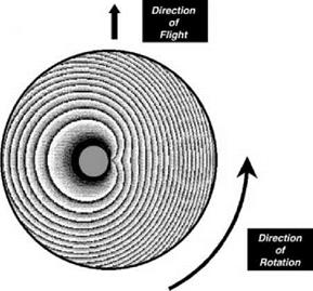
A blade is shown in Figure 4.2 at 90° and again at 270°. These are the positions of maximum and minimum relative air velocity normal to the blade, the velocities at the tip being (OR + V)and (OR—V), respectively. If the blade were to rotate at fixed incidence, then owing to this velocity differential, much more lift would be generated on the advancing side than on the retreating side. Calculated pressure contours for a fixed-incidence rotation with p = 0.3 are shown in Figure 4.3. For this situation, about four-fifths of the total lift is produced on the advancing side. The consequences of this imbalance would be large oscillatory bending stresses at the blade roots and a large rolling moment on the vehicle tending to roll the aircraft towards the retreating side. Both structurally and dynamically the helicopter would be unflyable.

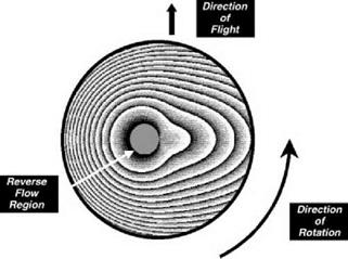
Clearly a cyclical variation in blade incidence is needed to balance lift on the two sides. If we permit the blade pitch to vary sinusoidally as the blade rotates around the azimuth to an amount which balances out the rolling moment of the rotor, the contours of pressure level for this roll – balanced lift distribution are of the type shown in Figure 4.4.

The mean pressure level is now lower, the lift on the advancing side being greatly reduced, with only small compensation on the retreating side. The fore and aft sectors now carry the main lift load. The total lift can be restored in some degree by applying a general increase in blade 1 Portions of this Chapter have been taken from The Foundations of Helicopter Flight by Simon Newman, Elsevier, 1994.

Basic Helicopter Aerodynamics, Third Edition. John Seddon and Simon Newman. © 2011 John Wiley & Sons, Ltd. Published 2011 by John Wiley & Sons, Ltd.

incidence level through the pilot’s control system (Section 4.3), but as this is performed the retreating blade, which is producing lift at relatively low airspeed, must ultimately stall. In addition, compressibility effects such as shock-induced flow separation must be considered, both on the advancing side where the Mach number is highest and on the retreating side where lower Mach number is combined with high blade incidence. Since the degree of load asymmetry across the disc increases with forward speed, the retreating-blade stall and its associated effects determine the maximum possible flight speed of the vehicle. For the conventional helicopter a speed of about 400 km/h (250 mph) is usually regarded as the upper limit.

While this technique would balance out the overall rolling moment, the rigid connection of the blades to the hub would cause a significant amount of vibratory forcing to be transmitted to the rotor hub and hence to the helicopter. The mechanisms which can avoid this are now described. The widely adopted method of achieving this is by use of flapping hinges, first introduced by Juan de la Cierva around 1923. The blade is freely hinged as close as possible to

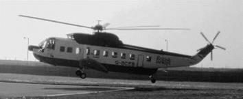
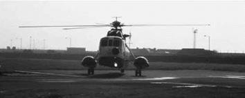
the root, allowing it to flap up and down out of the plane of rotation as it rotates about the rotor shaft. The presence of free hinges means that blade root stresses are avoided and no rolling moment is communicated to the airframe. The blades are now under the influence of two types of moments. The lift force is trying to flap the blades upwards by creating a moment about the flapping hinge – moving the blades out of the rotation plane – while the centrifugal force is working in opposition – driving the blades back towards the rotation plane. In hover, the blade position is stable and these two moments cancel out. Figure 4.5 shows a Sikorsky S61NM

hovering prior to landing. The rotor blades are ‘coned up’ as the flapping hinges relieve the flapping moment of the lift loads and the two moments are in equilibrium. Figure 4.6 shows the aircraft after touching down where the rotor thrust has been reduced to zero and the rotor disc is now flat, under the influence of the centrifugal effects only (gravity has a small effect which is usually neglected – the main rotor tip experiences centripetal accelerations of 750-1000 g).

As the rotor moves into horizontal flight the situation of Figure 4.2 establishes itself. The incident flow over the blades will depend on their azimuthal position. The blade on the advancing side experiences an increased incident flow and the lift will increase, overcoming the centrifugal moment, so the blade will now flap upwards. As it flaps upwards, a downward flow is superimposed on the blade and the lift will reduce. See Figure 4.7. This continues until the blade flaps to its highest position. The reverse effect occurs for the blade on the retreating side where the blade will flap downwards to its lowest position. The maximum velocity change is at the 90° and 270° azimuth. It will be shown that the extreme blade flapping angles are achieved very close to 90° of blade rotation around the azimuth. The result is that the blades will flap up at the front of the rotor and down at the rear and the disc will tilt rearwards. It is normally accepted that the thrust force is aligned with the normal to the rotor disc. We have the situation where the rotor thrust is now inclined rearwards and forward motion is not possible. In order for the rotor to supply forward propulsion, the rotor disc must be tilted forwards, directly opposing the natural effect of blade flapping. This can only be achieved by altering the blade lift through a pitch change. This is known as cyclic pitch and will be discussed later.

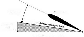Relative Wind from Forward Flight

Figure 4.7 Incident velocity components

This pitch angle movement is provided by a pitch bearing, known alternatively as the feathering hinge, linked to a control system operated by the pilot (Section 4.3).

An additional feature of the asymmetry in velocity across the disc is that there exists a region on the retreating side where the flow over the blade is actually reversed. At 270° azimuth the resultant velocity at a point r of span is:

U = O r-V

or non-dimensionally:

Thus the flow over the blade is reversed inboard of the point x = m. It will be apparent that the reversed flow boundary is a circle of diameter m, centred at x = m/2 on the 270° azimuth. Dynamic pressure in this region is low, so the effect of the reversed flow on the blade lift is small, usually negligible from a performance aspect for advance ratios up to 0.4. Very precise calculations may require the reversed flow region to be taken into account and it may be important also in studies of blade vibration. Some advanced rotor concepts have required the rotor rotational speed to be reduced, even halted. This will cause the reversed flow region to become a significant part of the rotor disc.

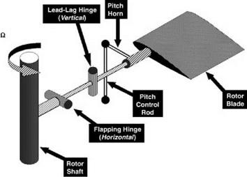
A flapping blade in rotation sets up Coriolis moments in the plane of the disc, and to relieve this it is usual to provide a second hinge, the lead-lag hinge, normal to the disc plane, allowing free in-plane motion. This may need to be fitted with a mechanical damper to ensure dynamic stability.

The standard articulated blade thus possesses this triple movement system of flapping hinge, lead-lag hinge and pitch bearing in a suitable mechanical arrangement, located inboard of the lifting blade itself. The principles are illustrated in Figure 4.8.

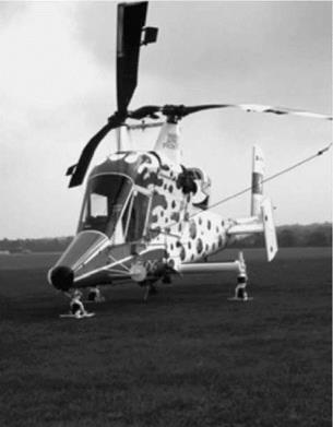
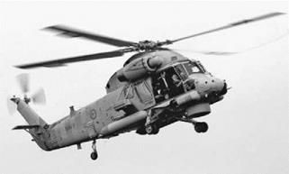
Kaman aircraft use a slightly different system where blade pitch is controlled by a trailing edge servo flap. This is deflected by the pilot’s controls, which generates a moment causing the blade to elastically bend in pitch. These servo flaps can be seen in Figure 4.9 which shows the KMax while Figure 4.10 shows the Seasprite.

Strictly the blade root bending stress and helicopter rolling moment are eliminated by flapping only if the hinge is located on the axis of rotation. This is impracticable for a rotor with more than two blades, so residual moments do exist. These are not important, however, if the offset of the hinge from the axis is only a few per cent of blade radius – which is normal. The flapping hinge is therefore normally made the innermost, with an offset of 3-4%. The lag hinge and pitch bearing can be more freely disposed: sometimes the former is the farther out of the two. The order of the hinges has a significant effect on the blade dynamic behaviour and if the pitch bearing is placed inboard of either or both of the flap and lag hinges, kinematic couplings can be generated.

The total mechanical complexity of an articulated rotor is substantial. Hinge bearings operate under high centrifugal loads, so service and maintenance requirements are severe. Hinges, dampers and control rods make up a bulky rotor head, which is likely to have a high parasitic drag – perhaps as much as the rest of the helicopter.

In modern rotors, the flapping and lag hinges are often replaced by flexible elements which allow the flapping and lead-lag motions of the blades to take place, albeit with a degree of stiffness not present with free hinges. With such hingeless rotors, bending stresses and rolling moments reappear, in moderation only but sufficient to modify the stability and control characteristics of the helicopter (Chapter 8). The effect of a flexible flapping element can usually be calculated by equating it to a hinged blade with larger offset (10-15%). The use of a hingeless rotor is one way of reducing the parasitic drag of the rotor head. A pitch bearing mechanism is of course needed for rotor control, as with the articulated rotor. The hingeless rotor of the Agusta Westland Lynx helicopter is pictured in Figure 4.11.

A characteristic of the actuator disc concept is that the linear theory of lift is maintained to the perimeter of the disc. Physically, as described in Chapter 2, we suppose the induced velocity, in which the pressure is above that of the surrounding air, to be contained entirely below the disc in a well-defined streamtube surrounded by air at rest relative to it. In reality, because the rotor consists of a finite number of separate blades, some air is able to escape outwards between the tips, drawn out by the tip vortices. Thus the total induced flow is less than the actuator disc theory would prescribe, so that for a given pitch setting of the blades the thrust is somewhat lower than that given by Equation 3.27. The deficiency is known as tip loss and is shown by a rapid falling off of lift over the last few per cent of span near the tip, in a typical blade loading distribution such as that of Figure 2.28.

Although several workers have suggested approximations [Bramwell (p. 111) quotes Prandtl, Johnson (p. 60) quotes in addition Sissingh and Wheatley], no exact theory of tip loss is available. A common method of arriving at a formula is to assume that outboard of a station r = BR the blade sections produce drag but no lift. Then the thrust integral in Equation 3.26 is replaced by (which is a change in the upper limit of the thrust integral, effectively ignoring the outer tip region of the blade):

whence is obtained, for uniform inflow and zero twist:

With a typical value B = 0.97 or 0.98 Equation 3.58 yields between 5% and 10% lower thrust than Equation 3.27 for a given value of O.

To obtain the effect on rotor power at a given thrust coefficient, we need to express the increase in induced velocity corresponding to the effective reduction of disc area. Since the latter is affected by a factor B2 and the induced velocity is proportional to the square root of disc loading (Equation 2.8), the increase in induced velocity is by a factor 1/B. The rotor induced
power in hover thus becomes:

= 1 (Ct)3/2 B ‘ 2

Typically this amounts to 2-3% increase in induced power. The factor can be incorporated in the overall value assumed for the empirical constant к in Equation 3.55.

3.6 Example of Hover Characteristics

Corresponding to CL/a and CD/CL characteristics for fixed wings, we have CT/0 and CP/CT for the helicopter in hover. An example has been evaluated using the following data:

The variation of CT/s with в is shown in Figure 3.8a. The nonlinearity results from the HCT term in Equation 3.32. The variation of CP/s with в is calculated for three cases:

• k = 1.13, Equation 3.55;

• k = 1.0, Equation 3.50, the simple momentum theory result;

• figure of merit M = 1.0, which assumes kj = 1.0 and CD0 = 0.

Over the range shown (Figure 3.8b), using the factor k = 1.13 results in a power coefficient 0-9% higher than that obtained using simple momentum theory. The curve for M = 1 is of course unrealistic but gives an indication of the division of power between induced and profile components.

(Rotor performance characteristics are sometimes plotted as CP/s versus CT/s. This type of plot is known as a hover polar.)

Reference

1. Glauert, H. (1983) The Elements of Aerofoil and Airscrew Theory, Reissued in the Cambridge Science Classics Series, Cambridge University Press.

From Equation 3.20 the differential power coefficient dCP (= dCQ) may be written as:

dCp — dCQ

= s(fCL + CD)x3 dx

— sCLf x3 dx + sCDx3 dx (3.46)

— sCL1x2 dx + sCDx3 dx

— dCpi + dCp0

where dCPi is the differential power coefficient associated with induced flow and dCP0 is that associated with blade section profile drag. The first term, using Equation 3.17, is simply:

whence:

Assuming uniform inflow and a constant profile drag coefficient CD0, we have the approximation:

Cp = l • Ct + -^ (3-50)

In the hover, where:

l = 1 УСТ (3.51)

this becomes:

Cp = 1 (Ct)3/2 + SC4D0 (3.52)

The first term of Equations 3.50 or 3.52 agrees with the result from simple momentum theory (Equation 2.12). The present l, defined by Equation 3.14, includes the inflow from climbing speed VC (if any), so the power coefficient term includes the climb power:

Pclimb = Vc • T (3.53)

The total induced power in hover or climbing flight is generally two or three times as large as the profile power. The chief deficiency of the formula in Equation 3.50 in practice arises from the assumption of uniform inflow. Bramwell (p. 94ff.) shows that for a linear variation of inflow the induced power is increased by approximately 13%. This and other smaller correction factors such as tip loss (Section 3.7) are commonly allowed for by applying an empirical factor kj to the first term of Equation 3.50, so that as a practical formula:

Cp = ki • l • Ct +(3-54)

is used, in which a suggested value of kj is 1.15. The combination of Equations 3.54 and 3.27 provides adequate accuracy for many performance problems.

For the hover, we have:

The figure of merit M may be written:

which demonstrates that for a given thrust coefficient a high figure of merit requires a low value of the product sCD0. Using a low solidity seems an obvious way to this end but it must be tempered because the lower the solidity, the lower the blade area, which means the higher the blade angles of incidence required to produce the thrust and the profile drag may then be increased significantly from either Mach number effects or the approach of stall. A low solidity, subject to retaining a good margin of incidence below the stall, would appear to be the formula for producing an efficient design.

For accurate performance work the basic relationships in Equations 3.18 and 3.21 are integrated numerically along the span. Appropriate aerofoil section data can then be used, including both compressibility effects and stalling characteristics. Further reference to numerical methods is made in Chapter 6.

Characteristics of a rotor obviously depend on the lift coefficient at which the blades are operating and it is useful to have a simple approximate indication of this. The blade mean lift coefficient provides such an indication. As the name implies, the mean lift is that which, applied uniformly along the blade span, would give the same total thrust as the actual blade. Writing the

mean lift coefficient as Cl we have, from Equation 3.18:

A

Clx2 dx

0

3sc l

from which:

The parameter CT/s has been previously discussed and this gives another reason for the preference some workers have for using it as the definition of thrust coefficient instead of CT.

Blades usually operate in the CL range 0.3-0.6, so typical values of CT/s are between 0.1 and 0.2. Typical values of CT are an order of 10 smaller as solidity values are in the region of 0.1.

Applying Equation 3.32 for the three-quarters radius point, at which У is 7.5°, gives a thrust coefficient CT = 0.0091. Turning now to Equation 3.36, the non-uniform l varies along the span as shown in Figure 3.5.

Superficially this is greatly different from a constant value – Equation 2.12. Nevertheless, on evaluating Equation 3.36 the variation of (Or2 — 1r) is as shown in the figure, from which the integrated value of thrust coefficient is CT = 0.0092. Thus the assumption of constant inflow has led to underestimating the thrust by a mere 1.7%. The result agrees well with Bramwell’s general conclusion (p. 93) and confirms that uniform inflow may be assumed for many, perhaps most, practical purposes.

3.2 Ideal Twist

The relation in Equation 3.36 contains one particular situation when l becomes a constant, that is if the term Ox is itself constant, then:

Ox — Otip

OTIP being the pitch angle at the tip. This nonlinear twist is not physically realizable near the root but the case is of interest because, as momentum theory shows, uniform induced velocity corresponds to minimum induced power. The analogy with elliptic loading for a fixed-wing aircraft is again recalled. The twist defined in Equation 3.37 is known as ideal twist. Inserting in

= Sa (-tip—l)

and, since l = xf = f TIP, the tip inflow angle, Equation 3.38 can be expressed as:

With ideal twist and the resulting constant value of l we find Equation 3.36 simplifies to:

and the direct relationship between – and CT is now:

-tip = 2 + Ct

sa 2

Some pitch angles for ideal twist and linear twist are compared in Figure 3.6.

The inboard end of the blade is assumed to be at r — 0, ignoring for the purposes of comparison the practical necessity of a root cutout. The linear twist is assumed to vary from 12° pitch at the root to 6° at the tip. Figure 3.7 shows a typical main rotor blade. The built-in twist is readily observed. A straightforward comparison is when the ideal twist has the same pitch at the tip—we see that unrealistically high pitch angles are involved at 40% radius and inboard. A more useful comparison is at equal thrust for the two blades. From Equations 3.32 and 3.41 it follows that for the same thrust coefficient the pitch angle at two-thirds span with the ideal twist is the same as that at three-quarters span with the linear twist, which for the case in point is 7.5°. Thus the ideal twist is given by:

This case is also shown in Figure 3.6. The two twist distributions give the same pitch angle when:

An assumption has been made so far, which is that the induced velocity is uniform across the rotor disc. This is an idealized situation, which in fixed-wing terms refers to the elliptically loaded wing which, itself, generates a uniform downwash. The effect of non-uniformity can be introduced by dividing the rotor disc into elements of concentric annuli, where we can treat each annulus as a lifting element and apply BET and momentum theory as before. By restricting the analysis to a generic annulus, over which the downwash can be considered constant, the restriction of uniformity of downwash can be removed. We restrict the analysis to hover and use

instead of l.

If we have an annulus of radius r and width dr, the thrust produced by this annulus can be expressed using BET, giving:

This thrust is expressed using momentum theory as:

dT = p • 2nr dr • Vi • 2Vi = 4ppr drV-2 = 4ppr dr(QR)2 • l2

Equating gives:

I

(3.36)

The inflow distribution may now be calculated as a function of x and the thrust evaluated from Equation 3.26.

As a numerical example let us consider the case of a blade having linear twist, from a collective pitch setting of 12° to 6° at the tip (the root cutout can be ignored for this purpose). The rotor solidity (s) is 0.08 and the lift curve slope value (a) is 5.7. The value of the pitch angle at 75% radius is then O75% = 7.5°.