Category BASIC HELICOPTER AERODYNAMICS

If the blade incidence a is measured from the no-lift line and stall and compressibility effects can be neglected, the section lift coefficient can be approximated by the linear relation:

Cl = aa = а(в—ф)

where the two-dimensional lift slope factor a has a value of about 5.7. Analyses of potential flow by Glauert [1] give a value for the lift curve slope of 2p per radian. The value of 5.7 is more representative allowing for losses due to viscous effects. This value also has the added benefit of being equivalent to 0.1 per degree. Equation 3.18 then takes the form:

(вх2—lx) dx

For a blade of zero twist, в is constant. For uniform induced velocity – as assumed in simple momentum theory – the inflow factor l is also constant. In these circumstances Equation 3.26 integrates readily to:

Conventionally, modern blades incorporate negative twist, decreasing the pitch angle towards the tip with the objective of evening out the blade loading distribution. Thus в takes a form such as:

в = во-кх (3.28)

Here, к is a linear twist expressed over the entire blade from rotor centre to blade tip. Modern blades can have twist variations which are nonlinear. Using this form, the thrust coefficient becomes:

The first two terms can be combined by introducing the blade pitch angle at 75% radius:

so the thrust coefficient becomes:

and the relation in Equation 3.27 is restored.

Thus a blade with linear twist has the same thrust coefficient as one of constant в equal to that of a linearly twisted blade at three-quarters radius.

Equation 3.27 expresses the rotor thrust coefficient as a function of pitch angle and inflow ratio. For a direct relationship between thrust coefficient and pitch setting, we need to remove the l term. This can be achieved by recalling the link between thrust and induced velocity provided by the momentum theorem.

For the rotor in hover, this is Equation 2.12, which on incorporation with Equation 3.27 leads to:

in which for a blade with a linear twist, в is taken at three-quarters radius. It is readily seen that correspondingly the direct relationship between в and l is:

(3.33)

3.1 Basic Method

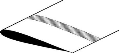
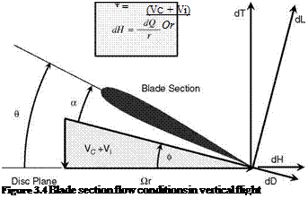
Blade element theory is basically the application of the standard process of aerofoil theory to the rotating blade. A typical aerodynamic strip is shown in Figure 3.1 and the appropriate notation for a typical strip is shown in Figure 3.2. Although in reality flexible, a rotor blade is assumed throughout to be rigid, the justification for this lying in the fact that at normal rotation speeds the outward centrifugal force is the largest force acting on a blade and, in effect, is sufficient to hold the blade in rigid form. In vertical flight, including hover, the main complication is the need to integrate the elementary forces along the blade span. Offsetting this, useful simplification occurs because the blade incidence and induced flow angles are normally small enough to allow small-angle approximations to be made.

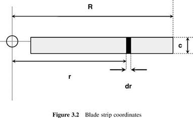
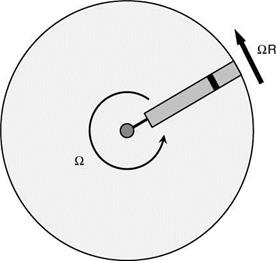
Figure 3.3 is a plan view of the rotor disc, seen from above. Blade rotation is anticlockwise (the normal system in the UK and the USA) with angular velocity Q. The blade radius is R, the tip speed therefore being QR, alternatively written as VT. An elementary blade section is taken at radius r, of chord length c and spanwise width dr. Forces on the blade section are shown in Figure 3.4. The flow seen by the section has velocity components Qr in the disc plane and (VC + Vi) perpendicular to it. The resultant of these is:

The blade pitch angle, determined by the pilot’s collective control setting (see Chapter 4), is У. The angle between the flow direction and the plane of rotation, known as the inflow angle, is f, given by:

Basic Helicopter Aerodynamics, Third Edition. John Seddon and Simon Newman. © 2011 John Wiley & Sons, Ltd. Published 2011 by John Wiley & Sons, Ltd.

or for small angles, which we shall assume:

The angle of incidence of the blade section, denoted by a, is seen to be:

a = 0—ф

The elementary lift and drag forces on the section are:

dL = 2 p U2 • c dr • CL

dD = pU2 • c dr • CD

Resolving these normal and parallel to the disc plane gives an element of thrust:

dT = dL cos ф—dD sin ф (3.6)

and an element of blade torque:

dQ = (dL sin ф + dD cos f)r (3.7)

The inflow angle ф may generally be assumed to be small; from Equation 3.3 this may be questionable near the blade root where Or is small, but there the blade loads are themselves small also. Masking the reasonable assumption that the rotor blade section has a high lift/drag

ratio, the following approximations can therefore be made:

U ‘ Or

dT ‘ dL (3.8)

dQ ‘ (f dL + dD)r

It is convenient to introduce dimensionless quantities at this stage. We write:

which leads to:

dCT = sCLx2 dx

Integrating along the blade span gives the rotor thrust coefficient as:

The rotor power requirement is given by:

P = OQ

Note that the power coefficient is defined as:

Hence CP and Cq are identical in value (essentially there is a O term multiplying both the numerator and denominator).

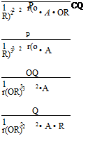
The definitions used in this book contain a half in the denominator. This is not universal as some analyses omit the half. It is also apparent that the normalizing factors are based, as in the lift coefficient, on a dynamic pressure and a reference area. The thrust, torque and power coefficients use the disc area. However, the introduction of blade element theory (BET) gives equations which feature the blade area, so another set of coefficients can be defined to reflect this:

T T Ct

2r(OR)2 • NcR 1 r(OR)2 • A •(NcR/A) s

Q_________________ Q__________ =Cq

2r(OR)2 • R • NcR 2r(or)2 • r • a • (NcR/A) s

P P________ Cp

1 r(OR)3 • NcR 1 r(OR)3 • A •(NcR/A) s

These are related to the original coefficients via the rotor solidity.

To evaluate Equations 3.18 and3.21 it is necessary to know the spanwise variation ofblade incidence a and to have blade section data which give Cl and Cd as functions of a. The equations can then be integrated numerically. Since a is given by (в — ф), its distribution depends upon the variations of в, the blade pitch, and (VC + V), the total induced velocity, represented by the inflow factor l. Useful approximations can be made, however, which allow analytical solutions with, in most cases, only small loss of accuracy.

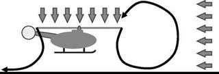
As the helicopter approaches the ground, the spreading wake will interact with any horizontal wind. This will tend to turn the upwind wake upwards after which it re-enters the rotor. This sets up a type of toroidal flow. The effect is shown schematically in Figure 2.33.

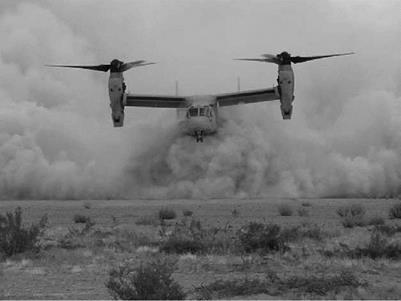
A considerable amount of research has been devoted to this effect, for the reason that when the helicopter is operating where the ground surface is easily raised into the air [13-15]. A cloud of ground debris is entrained by the interacting flows surrounding the aircraft. Visibility is severely restricted making operations very hazardous. Figure 2.34 shows a V22 descending into a cloud of dust caused by the downwash from the rotors.

References

1. Glauert, H. (1937) The Elements of Aerofoil and Airscrew Theory, Cambridge University Press.

2. Gustafson, F. B. and Gessow, A.(1945) Flight tests on the Sikorsky HNS-1 (Army YR-4B) helicopter, NACA MR L5D09a.

3. Gessow, A. (1948) Effect of rotor blade twist and planform taper on helicopter hovering performance, NACA Technical Notice 1542.

4. Brotherhood, P. and Stewart, W. (1949) An experimental investigation of the flow through a helicopter rotor in forward flight, ARC R&M 2734.

5. Castles, W. Jr and Gray, R. B. (1951) Empirical relation between induced velocity, thrust and rate of descent of a helicopter rotor as determined by wind tunnel tests on four model rotors, NACA TN 2474, October.

6. Jones, J. P. (1973) The rotor and its future. Aero. J., 751,77.

7. Gray, R. B. (1956) An aerodynamic analysis of a single-bladed rotor in hovering and low speed forward flight as determined from smoke studies of the vorticity distribution in the wake, Princeton University Aeronautical Engineering Report 356.

8. Landgrebe, A. J. (1972) The wake geometry of a hovering helicopter rotor and its influence on rotor performance. JAHS, 17(4), 3-15.

9. Landgrebe, A. J. (1971) Analytical and experimental investigation of helicopter rotor hover performance and wake geometry characteristics, USAAMRDL Technical Report, 71-24.

10. Clark, D. R. and Leiper, A. C. (1970) The free wake analysis – a method for the prediction of helicopter rotor hovering performance. JAHS, 15(1), 3-12.

11. Knight, M. and Hafner, R. A. (1941) Analysis of ground effect on the lifting airscrew, NACATN 835.

12. Cheeseman, I. C. and Bennett, W. E. (1955) The effect of the ground on a helicopter rotor, ARC R & M 3021.

13. Phillips, C., Kim, H. W. and Brown, R. E. (2009) The effect of rotor design on the fluid dynamics of helicopter brownout. 35th European Rotorcraft Forum, Hamburg, September.

14. Phillips, C., Kim, H. W. and Brown, R. E. (2010) Helicopter brownout – can it be modelled? RAeS Rotorcraft Group Conference ‘Operating Helicopters Safely in a Degraded Visual Environment’, London, June.

15. Phillips, C., Kim, H. W. and Brown, R. E. (2010) The flow physics of helicopter brownout. 66th American Helicopter Society Annual Forum, Phoenix, AZ, May.

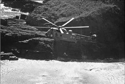
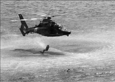
The induced velocity of a rotor in hover is considerably influenced by the near presence of the ground. At the ground surface the downward velocity in the wake is, of course, reduced to zero and this effect is transferred upwards to the disc through pressure changes in the wake, resulting in a lower induced velocity for a given thrust. This is shown in Figures 2.30 and 2.31.

The two images illustrate the wake impinging on the water during air sea rescue operations. The outward motion of the waves shows how the vertical velocity at the rotor disc is turned to a horizontal direction by the effect of the sea. The induced power is therefore lower, which is to say that a helicopter at a given weight is able to hover at lower power thanks to ‘support’ given by the ground. Alternatively put, for a given power output, a helicopter ‘in ground effect’ is able to hover at a greater weight than when it is away from the ground. As Bramwell has put it, ‘the improvement in performance may be quite remarkable; indeed some of the earlier, under­powered, helicopters could hover only with the help of the ground’.

The theoretical approach to ground effect is, as would be expected, by way of an image concept. A theory by Knight and Hafner [11] makes two assumptions about the normal wake:

1. That circulation along the blade is constant, thus restricting the vortex system to the tip

vortices only.

2. That the helical tip vortices form a uniform vortex cylinder reaching to the ground.

The ground plane is then represented by a reflection of this system, of equal dimensions below the plane but of opposite vorticity, ensuring zero normal velocity at the surface. The induced velocity at the rotor produced by the total system of real and image vortex cylinders is calculated and hence the induced power can be derived as a function of rotor height above the ground.

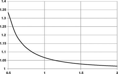
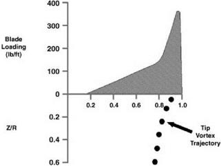
It is found that the power, expressed as a proportion of that required in the absence of the ground, is as low as 0.5 when the rotor height to rotor radius is about 0.4, a typical value for the point of take-off. Since induced power is roughly two-thirds of total power (Section 2.1), this represents a reduction of about one-third in total power. By the time the height to radius ratio reaches 2.0, the power ratio is close to 1.0, which is to say ground effect has virtually disappeared. The results are only slightly dependent on the level of thrust coefficient.

Similar results have been obtained from tests on model rotors, measuring the thrust that can be produced for a given power. A useful expression emerges from a simple analysis made by Cheeseman and Bennett [12], who give the approximate relationship:

where T is the rotor thrust produced in ground effect and T1 is the rotor thrust produced out of ground effect at the same level of power. Z is the rotor height above the ground and R is the rotor radius. The variation is shown in Figure 2.32.

This shows good agreement with experimental data.

Ground effect has a profound influence on a helicopter’s performance and so a technical specification will often include two values for a quantity such as power or thrust either in ground effect (IGE) or out of ground effect (OGE).

By analysis of his carefully conducted series of smoke-injection tests, Landgrebe [9] reduced the results to formulae giving the radial and axial coordinates of a tip vortex in terms of azimuth angle, with corresponding formulae for the inner sheet. From these established vortex positions (the so-called prescribed wake) the induced velocities at the rotor plane may be calculated. The method belongs in a general category of prescribed-wake analysis, as do earlier analyses by Prandtl, Goldstein and Theodorsen, descriptions of which are given by

Bramwell. These earlier forms treated either a uniform vortex sheet as pictured in Figure 2.25 or the tip vortex in isolation, and so for practical application are effectively superseded by Landgrebe’s method.

More recently, considerable emphasis has been placed on free-wake analysis, in which modern numerical methods are used to perform iterative calculations between the induced – velocity distribution and the wake geometry, both being allowed to vary until mutual

consistency is achieved. This form of analysis has been described for example by Clark and Leiper [10]. Generally the computing requirements are very heavy, so consid­erable research effort also goes into devising simplified free-wake models which will reduce the computing load. The computing power available is consistently increasing with time; however, the complexity of the methods always seems to fill the available computing capability.

Calculations for a rotor involve adding together calculations for the separate blades. Generally this is satisfactory up to a depth of wake corresponding to at least two rotor revolutions. A factor which helps this situation is the effect on the tip vortex of the upwash ahead of the succeeding blade – analogous to the upwash ahead of a fixed wing. The closer the spacing between blades, the stronger the effect from a succeeding blade on the tip vortex of the blade ahead of it; thus it is observed that when the number of blades is large, the tip vortex remains approximately in the plane of the rotor until the succeeding blade arrives, when it is convected downwards. In the ‘far’ wake, that is beyond a depth corresponding to two rotor revolutions, it is sufficient to represent the vorticity in simplified fashion; for example, free – wake calculations can be simplified by using a succession of vortex rings, the spacing of which

is determined by the number of blades and the mean local induced velocity. Eventually in practice both the tip vortices and the inner sheets from different blades interact and the ultimate wake moves downwards in a confused manner.

There we leave this brief description of the real wake of a hovering rotor and the methods used to represent it. This branch of the subject is often referred to as vortex theory. It will be touched on again in the context of the rotor in forward flight (Chapter 5). For more detailed accounts, the reader is referred to the standard textbooks and the more specific references which have been given in these past two sections.

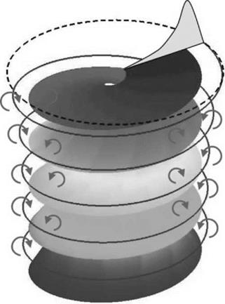
The actuator disc concept, taken together with blade element theory, serves well for the purposes of helicopter performance calculation. When, however, blade loading distributions or vibration characteristics are required for stressing purposes, it is necessary to take into account the real nature of flow in the rotor wake. This means abandoning the disc concept and recognizing that the rotor consists of a number of discrete lifting blades, carrying (bound) vorticity corresponding to the local lift at all points along the span. Corresponding to this bound vorticity, a vortex system must exist in the wake (Helmholtz’s theorem) in which the strength of wake vortices is governed by the rate of change of circulation along the blade span. If for the sake of argument this rate could be made constant, the wake for a single rotor blade in hover would consist of a vortex sheet of constant spanwise strength, descending in a helical pattern at constant velocity, as illustrated in Figure 2.25. The situation is analogous to that of elliptic loading with a fixed wing, for which the induced drag (and hence the induced power) is a minimum. This ideal distribution of lift, however, is not realizable for the rotor blade, because of the steadily increasing velocity from root to tip.

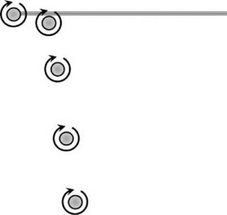
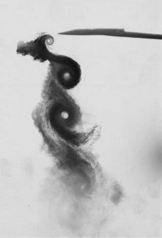
The most noticeable feature of the rotor blade wake in practice is the existence of a strong vortex emanating from the blade tip where, because the velocity is highest, the rate of change of lift is greatest. In hover, the tip vortex descends below the rotor in a helical path.

This can be visualized in a wind tunnel using smoke injection (Figure 2.26) or other means and is often observable in open flight under conditions of high load and high humidity. An important feature which can be seen in Figure 2.27 is that on leaving the blade the tip vortex initially moves inwards towards the axis of rotation and stays close under the disc plane; in consequence the next tip to come round receives an upwash, increasing its effective incidence and thereby intensifying the tip vortex strength.

Figure 2.28 due to J. P. Jones [6] shows a calculated spanwise loading for a Wessex helicopter blade in hover and indicates the tip vortex position on successive passes. The kink in loading distribution at 80% span results from this tip vortex pattern, particularly from the position of the immediately preceding blade.

The concentration of the tip vortex can be reduced by design changes such as twisting the tip nose-down, reducing the blade tip area or special shaping of the planform, but it must be borne in mind that the blade does its best lifting in the tip region where the velocity is high.

Since blade loading increases from the root to near the tip (Figure 2.28), the wake may be expected to contain some inner vorticity in addition to the tip vortex. This might appear as a form of helical sheet akin to that of the illustration in Figure 2.25, though generally not of uniform strength. Definitive experimental studies by Gray [7], Landgrebe [8] and their associates have shown this to be the case. Thus the total wake comprises essentially the strong tip vortex and an inner vortex sheet, normally of opposite sign. The situation as established by Gray and Landgrebe is pictured, in a diagram which has become standard, by Bramwell (p. 117) and other authors.

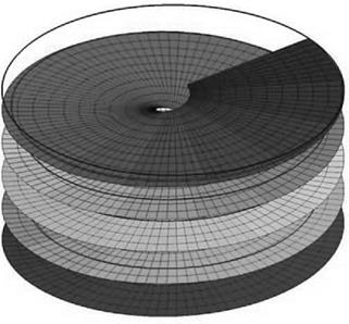
Figure 2.29 is a modified version of this diagram, intended to indicate the inner vorticity sheet, emanating from the bound vorticity on the inner part of the blade.

The Gray and Landgrebe studies show clearly the contraction of the wake immediately below the rotor disc. Other features which have been observed are that the inner sheet moves downwards faster than the tip vortex and that the outer part of the sheet moves faster than the inner part, so the sheet becomes increasingly inclined to the rotor plane.

The place of momentum theory is that it gives a broad understanding of the functioning of the rotor and provides basic relationships for the induced velocity created and the power required in

producing a thrust to support the helicopter. The actuator disc concept, upon which the theory is based, is most obviously fitted to flight conditions at right angles to the rotor plane, that is to say the hover and axial flight states we have discussed. Nevertheless, further reference to the theory will be made when discussing forward flight (Chapter 5).

Momentum theory brings out the importance of disc loading as a gross parameter; it cannot, however, look into the detail of how the thrust is produced by the rotating blades and what design criteria are to be applied to them. For such information we need additionally a blade element theory, corresponding to aerofoil theory in fixed-wing aerodynamics. We shall turn to this in Chapter 3.

The point of intersection of the induced-velocity curve with the line:

Vc + Vi = 0 (2.60)

is of particular interest because it defines what is termed the state of ideal autorotation[4] (IA in Figure 2.22), in which, since there is no mean flow through the rotor, the induced power is zero.

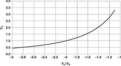
In round terms, values of Vc/V0 for ideal and real autorotation are about —1.7 and —1.8, respectively.

Pursuing the analogy of flow past a solid plate (turbulent wake state), the plate drag may be written:

1 2

D = – rVC • A • Cd

and if this is equated to rotor thrust we have:

from which we find:

(2.63)

Examining Figure 2.24, we see that with Vc/V0 = —1.7, Cd has the value 1.38 which is close to that for a solid plate. A slightly better analogy is obtained by taking the real value Vc/V0 =—1.8, which yields a Cd value of 1.23, close to the effective drag coefficient of a parachute.

Thus in autorotative vertical descent the rotor behaves like a parachute.

Equation 2.30 shows the power required to climb and generate downwash. To this is added the profile power. If we examine the equivalent power consumption in descent we find the following equation:

P = T (-VD + Vi)+ Pp = – T • Vd + T • Vi + Pp

The profile power expression is independent of the climb/descent speed so the hover result (Equation 2.16) is applicable here. Equation 2.58 now has the possibility of attaining the value zero. This would mean that no power input to the engine is required. Assuming this to be the situation, we have the following expression:

(2.59)

While this is the simplest form, with no factors applied, it illustrates the importance of disc loading – hence downwash – in the descent rate that is required to establish this condition of no
power input. This is the autorotation condition used by helicopters to land safely when power to the main rotor is lost. It is not surprising that this autorotation speed is kept as low as possible, so the downwash should be limited in value. This places a minimum limit on the main rotor radius.

2.9.1 Basic Envelope

It is of interest to know how the induced velocity varies through all the phases of axial flight. For the vortex ring and turbulent wake states, where momentum theory fails, information has been obtained from measurements in flight, supported by wind tunnel tests [2-5]. Obviously the making of flight tests (measuring essentially the rate of descent and control angles) is both difficult and hazardous, especially where the vortex ring state is prominent, and not surprisingly the results (see Figure 2.21) show some variation. Nevertheless the main trend has been ascertained and what is effectively a universal induced-velocity curve can be defined.

HOVERFLY I BY BLADE

1.0

/PROPORTIONAL TO AXIALY

VELOCITY OF ROTOR

Figure 2.21 Experimental test results for axial flight

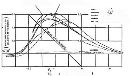
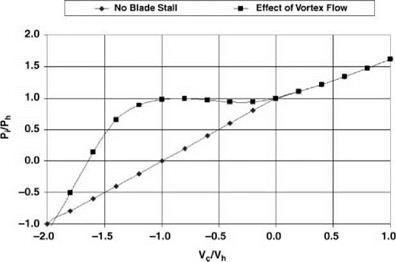
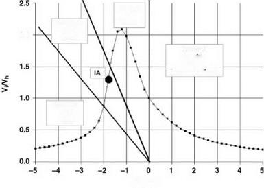This is shown in Figure 2.22, using the simple momentum theory results of Equation 2.55 in the regions to which they apply. We see that on moving from hover into descent the induced velocity increases more rapidly than momentum theory would indicate. The value rises, in the vortex ring state, to about twice the hover value, then falls steeply to about the hover value at entry to the windmill brake state.

The power required to maintain thrust in vertical descent generally falls as the rate of descent increases, except that in the vortex ring state an increase is observed (Figure 2.23). The effect appears to be caused by stalling of the blade sections during the violent vortex-shedding action. The increase can be potentially hazardous when making a near-vertical landing approach under conditions in which the engine power available is relatively low, as would be the case under high helicopter load in a high ambient temperature.