Category THEORETICAL AERODYNAMICS

The lift coefficient for an aerofoil in terms of the circulation k0 around it, by Equation (8.6a), is:

nbk0

Cl —

The aspect ratio of the aerofoil is:

_ span 2b яі — — —

chord c

2b x 2b c x 2b _ 4b2

— ~y.

ко

4b

Thus, the lift coefficient in terms of constant downwash velocity, at the trailing edge, is:

лЛію

U

By Equation (8.3), w/U = e and by Equation (8.25):

є = (a — a0).

Therefore:

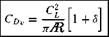
By Equation (8.8), the induced drag coefficient is:

C2

Cl

nJR

The variation of Cl with CDv is called the polar curve of the aerofoil.

Equation (8.8) shows that the polar curve of an elliptically loaded aerofoil is a parabola, provided the only source of the drag is the induced velocity.

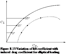The polar curve is as shown in Figure 8.13. The polar curve can be graduated in incidence as indicated in Figure 8.13. Since a is proportional to the lift coefficient Cl, equal increments of incidence gradients of the polar correspond to equal increment of Cl.

For incidence below the stall, the CL verses a curves are straight lines whose slopes increase as the aspect ratio increases, as shown in Figure 8.14.

For an elliptical load, as shown in Figure 8.4, the (k(y), y) curve is an ellipse. If P is a point on the span whose eccentric angle is в, we have y = —b cos в and therefore:

k(y) = k0 sin в, (8.30)

where k0 is the value of k(y) at y = 0. It is easily seen that the elimination of в gives:

which is an ellipse.

Substituting y = —b cos ф in Equation (8.15), the downwash velocity at the trailing edge is:

Thus for elliptic loading, the downwash velocity is the same at every point on the trailing edge. Now, by substituting Equation (8.28) into Equation (8.29), we get:

where a0′ and a’ refer to the section at distance y from the plane of symmetry.

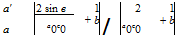
The chord c’ and incidence a’ depend, in general, on the particular profile section considered, that is on в. Also k0/V depends on the incidence of the aerofoil. If we increase the incidence of the aerofoil by в, the incidence of each profile section will also increase by в. Thus:

2 sin в 1

~—Г + 7

c a.0 b

where (ki) denotes the new value of Vi. From Equations (8.32) and (8.33), we get:

	2 sin в	1
	c’a0′	b

k0 V

= в.

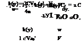
where c0 is the chord of the middle section of the aerofoil (that is, at y = 0), and a0′ will be same at every section and Equation (8.34) becomes:

c’ = c0 sin в.

This implies that the plot of chord c’ against y is also an ellipse. This situation can be realized by an aerofoil so constructed that its planform is bounded by two half ellipses whose major axis is equal to the span of the aerofoil. This can be proved by using the ellipses:

It follows that:

X1 _ X2 _ X1 ± X2 a1 a2 a1 ± a2

and if C — x1 ± x2, c0 — a1 ± a2, Equation (8.35) is satisfied.

Finally, it is evident from Equations (8.32) and (8.34) that for elliptic loading, which remains elliptic for all incidences, the incidence is the same at every profile section, and k0 is proportional to the incidence, and therefore, from Equation (8.31), the downwash is proportional to the incidence.

Another case arises for an aerofoil of rectangular planform. Here the chord c’ may be taken as constant and equal to c0. Retaining the hypothesis that a0′ — a0, which will be true if the sections are similar, or if they are thin, Equation (8.32) becomes:

This shows that the incidence at each section is different, so that the aerofoil is twisted. The incidence at the middle section will be a, got by assigning в — n/2 in Equation (8.36), and therefore:

(8.37)

Equation (8.37) shows that if the loading is elliptic at the incidence a, it ceases to be elliptic at a different incidence.

For an aerofoil:

• Geometrical incidence is the angle between the chord of the profile and the direction of motion of the aerofoil.

• Absolute incidence is the angle between the axis of zero lift of the profile and the direction of motion of the aerofoil.

When the axes of zero lift of all the profiles of the aerofoil are parallel, each profile meets the freestream wind at the same absolute incidence, the incidence is the same at every point on the span of the aerofoil, and the aerofoil is said to be aerodynamically untwisted.

An aerofoil is said to have aerodynamic twist when the axes of zero lift of its individual profiles are not parallel. The incidence is then variable across the span of the aerofoil.

To distinguish between the lift and induced drag coefficients and the incidences of the aerofoil (that is, wing) as a whole and its individual profiles, let us use CL, CDv, a for the aerofoil and CL’, CDv’, a’ for an individual profile. The coefficients CL’, CDv’ and a’ for a profile are functions of the coordinate y which defines the position of the profile. For a symmetrical aerofoil they are even functions of y, that is, to say that they are the same for +y and — y.

The lift and induced drag coefficients of the profile can be expressed as:

1 pV2 c dyC L = pVT(y)dy 2 pV2c’dyCDv’ = pwY(y)dy.

Therefore the drag and lift ratio becomes:

(8.24)

For a properly designed profile, the ratio of induced drag to lift is always small in the working range of incidence, and therefore A, which is called the angle of downwash, is a small angle. It follows that if V’2 = V2 + w2 then V = V, neglecting the second order of small quantities.

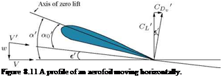As shown in Figure 8.11, the resultant aerodynamic force on the strip is perpendicular to the direction of V and not to the direction of V. Since e’ is a small angle, the coefficient of this force is CL’. Therefore in respect to lift the strip (profile) behaves like a strip of a two-dimensional aerofoil in a relative wind in the direction of V’, that is at incidence a0′, where:

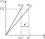
Figure 8.12 Profile lift coefficient variation with incidence (a) for a two-dimensional aerofoil, (b) for a three­dimensional aerofoil.

The angle a0′ is called the effective incidence. Thus the effective downwash is the downwash velocity that combines with the actual relative wind of speed V to produce an effective relative wind in the direction of V’.

The lift coefficient CL’ variation with incidence will be as shown by curve a in Figure 8.12. This curve is the graph proper to the profile operating as a two-dimensional aerofoil and the lift curve slope is given by:

, CL’ a0 = —: • a#0

But when the profile is operating as a part of the actual wing (that is, a three-dimensional aerofoil), the variation of CL’ with incidence will be as shown by curve b in Figure 8.12. The lift curve slope is given by:

CL

da’

It is seen that the graphs of CL’ against incidence are straight lines. In Figure 8.12, the graphs a and b are drawn with the assumption that the angle of downwash vanishes when the wind is along the axis of zero lift, that is, the axis of zero lift is assumed to be the same in the two-dimensional and three-dimensional aerofoils. With this assumption we have:

CL = a0 a0 = a! a’ • (8^26)

We know that for an actual aerofoil in a subsonic flow the main components of the drag are the profile drag and the skin friction drag. The induced drag caused by the downwash is an additional component of drag. Therefore, the total drag coefficient of the strip (profile), using Equation (8.24), is:

CD = CDo’ + c’Cl’, (827)

where CD0′ is the coefficient of profile drag for the profile.

It may be noted that the profile drag is largely independent ofincidence in the working range. Profile drag is the sum of the skin friction due to viscosity, and form drag due to the shape. The part due to skin friction is due to the no-slip caused by the viscosity of the air in the boundary layer at the surface of the body. This viscous effect is always present, but can be reduced by smoothening the surface and reducing the surface area.

The form drag due to the shape is owing to the high pressure at the leading edge and low pressure at the trailing edge (that is the low pressure in the wake). By shaping the body to reduce the wake to be of negligible thickness, that is by streamlining, the form drag can be almost eliminated.

Therefore:

This is the integral equation from which circulation k(y) is to be determined. Using this k(y), the lift, drag, and downwash can be determined.

Note that in general a’, a0′, C’ are functions of y, since incidence, chord and profile may vary from section to section. If the profiles are similar curves, a0′ is the same at every section, but a’ is not the same unless the sections are also similarly situated (untwisted aerofoil).

For a given wing a0′ a0′, c’ are known functions of y, and in particular for thin wings we may assume a0′ = 2n.

The following are the two problems associated with aerofoils:

• For a given circulation k(y), the form of the aerofoil and the induced drag are to be determined.

• For a given form of aerofoil, the distribution of circulation and the induced drag are to be determined.

It is a representation to improve on the accuracy of the horseshoe vortex system. In lifting line theory, the bound vortex is assumed to lie on a straight line joining the wing tips (known as lifting line). Now the vorticity is allowed to vary along the line. The lifting line is generally taken to lie along the line joining the section quarter-chord points of the wing. The results obtained using this representation is generally good provided that the aspect ratio of the wing is moderate or large, generally not less than 4.

Consider the lifting line as shown in Figure 8.10. At any point on the lifting line, the bound vortex is T(y), and there is consequently trailing vorticity of strength dT/dy per unit length shed. Note that T(y) is used to represent vortex distribution, instead of k(y). This is because it is a common practice to use both k(y) and T(y) to represent the vortex distribution.

The velocity induced by the elements of trailing vorticity of strength (dT/dy).dy at point p is given

by:

1 (dT/dy)

— ———– dy.

4n y1 – y

Total downwash at point P1 is:

The assumption in this analysis is that the downwash velocity w is small compared to the freestream velocity V, so that w/V is equal to the downwash angle e.

Let ae (y1) be the effective angle of incidence of the wing section at point Pj. The geometrical incidence of the same section be a(y). Let both these angles be measured from the local zero-lift angle. Then:

If a<x, is the lift-curve slope of the wing section at point Pj, which may also vary across the span, the local lift coefficient CL is given by:

Ci(yi) = axae(yi).

For the vortex drag Dv to be minimum, the S in Equation (8.13) must be zero. That is, X (or a) must be zero so that the distribution for Dv minimum becomes:

к = k)

=^.

This is an ellipse, thus the vortex distribution for drag minimum is semi-ellipse. The minimum drag distribution produces a constant downwash along the span while all other distributions produce a spanwise variation in induced velocity, as illustrated in Figure 8.9.

It is seen that the elliptic distribution gives constant downwash and minimum drag, non-elliptic distri­bution gives varying downwash.

If the lift for the aerofoils with elliptical and non-elliptical distribution is the same under given con­ditions, the r

(c) equivalent variation of downwash.

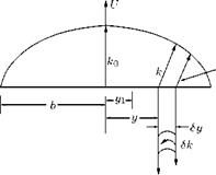
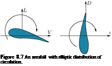
The spanwise variation in circulation is taken to be represented by a semi-ellipse having the span (2b) as the major axis and the circulation at the mid-span (k0) as the semi-minor axis, as shown in Figure 8.4, will have the lift and induced drag acting on it as shown in Figure 8.7.

From the general expression for an ellipse, shown in Figure 8.4, we have:

+ У = 1

or

(8.5)

This is the expression k = f (y) which can Aerofoil Characteristic with a More General Distribution

A more general distribution must satisfy the end conditions, namely, at the wing tips the vorticity should be zero. That is:

At y = ±b k = 0.

It is found that, for plain rectangular or slightly tapered aerofoils, the spanwise distribution does not depart drastically from elliptic distribution. The modified elliptic loading can satisfy this situation. Let:

1 + a{b

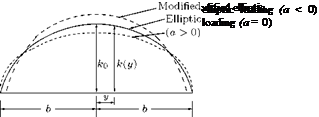The constant a can vary positively or negatively and therefore, can change the shape, but the end conditions are satisfied, as illustrated in Figure 8.8. In this figure, the area enclosed by the curves for a < 0, a = 0 and a > 0 are the same. That is, the total lift for elliptic and modified elliptic loading in this figure are the same.

8.4 The Vortex Drag for Modified Loading

The vortex drag, by Equation (8.4), is:

f Ь

Dv = pwkdy.

But for modified loading, the downwash, by Equation (8.11), is:

1 – 2k + 12k ( — b

and the vortex distribution is:

2

k = M/1 –

Substituting for w and k, we get the vortex drag as:

2	M/1 -( bj II + 4k(b) ) dy.
Dv
1 – 2k + 12k ( — b

The load is symmetrical about the mid plane, therefore the limits can be written as:

D=2 f‘ £ [‘- 2k+12k (b Я ‘V1 – (b)! (‘+4k (y)!) *.

Let y = b sin ф, therefore, dy = b cos фdф and the limits become 0 and n/2. Hence:

= —-° / [(1 – 2k) cos2 ф + (16k – 8k2) sin2 ф cos2 ф

+ 48k2 sin4 ф cos2 ф] dф.

These are standard integrals which result as:

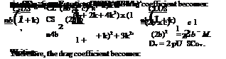
the drag coefficient can be expressed as:

(8.13)

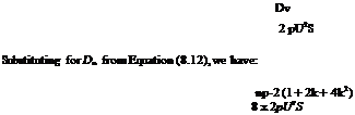
This drag coefficient for the modified loading is more than that for elliptical loading by an amount S, which is always positive since it contains X2 terms only.

Let us consider the aerofoil with hypothetical spanwise variation of circulation due to the combined bound vortex filaments as shown in Figure 8.4. At some point y along the span, an induced velocity equal to:

f ‘(y)dy 4n(y — yO ‘

will be felt in the downward direction. All elements shed vorticity along the span and add their contribution to the induced velocity at y1 so that the total influence of the trailing system at y1 is:

_ 1 rb ГШу

Wyl 4n J—b (y — y1) ’

Figure 8.3 Spanwise distribution of bound vortex filaments.

Figure 8.4 Spanwise variation of the strength of the combined bound vortex filaments.

Sk

w

Figure 8.5 Variation of downwash caused by the vortex system around an aerofoil.

that is:

The induced velocity at y1, in general, is in the downward direction and is called downwash.

The downwash has the following two important consequences which modify the flow about the aerofoil and alter its aerodynamic characteristics:

• The downwash at y1 is felt to a lesser extent ahead of y1 and to a greater extent behind, and has the effect of tilting the resultant wind at the aerofoil through an angle:

(8.3)

The downwash around an aerofoil will be as illustrated in Figure 8.5.

The downwash reduces the effective incidence so that for the same lift as the equivalent infinite or two-dimensional aerofoil at incidence a, an incidence of a = a^ + e is required at that section of the aerofoil. Variation of downwash in front of and behind an aerofoil will be as shown in Figure 8.5. As illustrated in Figure 8.5, the downwash will diminish to zero at locations far away from the leading edge and will become almost twice of its magnitude wcp at the center of pressure, downstream of the trailing edge.

• In addition to this motion of the air stream, a finite aerofoil spins the air flow near the tips into what eventually becomes two trailing vortices of considerable core size. The generation of these vortices requires a quantity of kinetic energy. This constant expenditure of energy appears to the aerofoil as the trailing vortex drag.

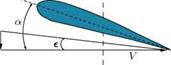
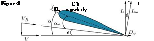
Figure 8.6 shows the two velocity components of the relative wind superimposed on the circulation generated by the aerofoil. In Figure 8.6, LOT is the two-dimensional lift, VR is the resultant velocity and V is the freestream velocity. Note that the two-dimensional lift is normal to VR and the actual lift L is normal to V. The two-dimensional lift is resolved into the aerodynamic forces L and Dv, respectively, normal and against the direction of the velocity V of the aerofoil. Thus, an important consequence of the downwash is the generation of drag Dv. Also, as illustrated in Figure 8.6, the vortex system inducing downwash w tilts the aerofoil in the nose-up direction. In Figure 8.6, V is the forward speed of aerofoil, VR is the resultant velocity at the aerofoil, a is the incidence, e (= w/V) is the downwash angle, aOT = (a — e), the equivalent two-dimensional incidence and Dv is the trailing vortex drag. The trailing vortex drag is also referred to as vortex drag or induced drag.

The forward wind velocity generates lift and the downwash generates the vortex drag Dv:

This shows that there is no vortex drag if there is no trailing vorticity.

As a consequence of the trailing vortices, which are produced by the basic lifting action of a (finite span) wing, the wing characteristics are considerably modified, almost always adversely, from those of the equivalent two-dimensional wing of the same section. A wing whose flow system is closer to the two-dimensional case will have better aerodynamic characteristics than the one where the end effects are conspicuous. That is, large aspect ratio aerofoils are better than short span aerofoils.

8.1 Introduction

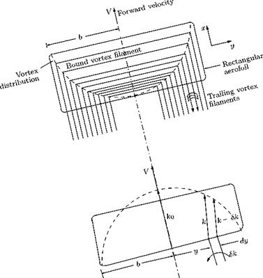
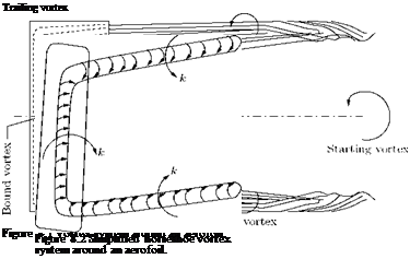
The vortex theory of a lifting aerofoil proposed by Lancaster and the subsequent development by Prandtl made use of for calculating the forces and moment about finite aerofoils. The vortex system around a finite aerofoil consists of the starting vortex, the trailing vortex system and the bound vortex system, as illustrated in Figure 8.1.

The horseshoe vortex system around an aerofoil, consisting of the bound and trailing vortices, can be simplified as shown in Figure 8.2.

8.2 Relationship between Spanwise Loading and Trailing Vorticity

From Helmholtz’s second theorem, the strength of the circulation around any section of a bundle of vortex tubes is the sum of the strength of the vortex filaments cut by the section plane. As per this theorem, the spanwise variation of the strength of the combined bound vortex filaments may be shown as illustrated in Figure 8.3.

If the circulation curve can be described as some function of y, say f (y), then the strength of the circulation shed by the aerofoil becomes:

that is:

Sk = – f'(y) dy. (8.1)

Now at a section of the aerofoil the lift per unit span is given by:

l = pUk,

where p and U are the density and velocity of the freestream. Thus, for a given flight speed and flow density, the circulation strength k is proportional to l. From the above discussion, it can be inferred that:

• The trailing filaments are closer showing that the vorticity strength is larger near the wing tips than other locations. That is, near the wing tips, the vorticity content of the vortices shed are very strong.

• Aerofoils with infinite span (b ^ to) or two-dimensional aerofoils will have constant spanwise loading.

Theoretical Aerodynamics, First Edition. Ethirajan Rathakrishnan.

© 2013 John Wiley & Sons Singapore Pte. Ltd. Published 2013 by John Wiley & Sons Singapore Pte. Ltd.

The major steps to be followed in the use of panel methods are:

• Vary the size of panels smoothly.

• Concentrate panels where the flow field and/or geometry is changing rapidly.

• Don’t spend more money and time (that is, numbers of panels) than required.

Panel placement and variation of panel size affect the quality of the solution. However, extreme sensi­tivity of the solution to the panel layout is an indication of an improperly posed problem. If this happens, the user should investigate the problem thoroughly. Panel methods are an aid to the aerodynamicist. We must use the results as a guide to help us and develop our own judgement. It is essential to realize that the panel method solution is an approximation of the real life problem; an idealized representation of the flow field. An understanding of aerodynamics that provides an intuitive expectation of the types of results that may be obtained, and an appreciation of how to relate your idealization to the real flow is required to get the most from the methods.

7.5.1 Limitations of Panel Method

0. Panel methods are inviscid solutions. Therefore, it is not possible to capture the viscous effects except via user “modeling” by changing the geometry.

1. Solutions are invalid as soon as the flow develops local supersonic zones [that is, Cp < CpJ. For two-dimensional isentropic flow, the exact value of Cp for critical flow is:

CPcri

7.5.2 Advanced Panel Methods

So-called “higher-order” panel methods use singularity distributions that are not constant on the panel, and may also use panels which are nonplanar. Higher order methods were found to be crucial in obtaining accurate solutions for the Prandtl-Glauert Equation at supersonic speeds. At supersonic speeds, the Prandtl-Glauert equation is actually a wave equation (hyperbolic), and requires much more accurate numerical solution than the subsonic case in order to avoid pronounced errors in the solution (Magnus and Epton). However, subsonic higher order panel methods, although not as important as the supersonic flow case, have been studied in some detail. In theory, good results can be obtained using far fewer panels with higher order methods. In practice the need to resolve geometric details often leads to the need to use small panels anyway, and all the advantages of higher order panelling are not necessarily obtained. Nevertheless, since a higher order panel method may also be a new program taking advantage of many years of experience, the higher order code may still be a good candidate for use.

Example 7.1

Discuss the the main differences of panel method compared to thin aerofoil theory and compile the essence of panel method.

Solution

Although thin airfoil theory provides invaluable insights into the generation of lift, the Kutta-condition, the effect of the camber distribution on the coefficients of lift and moment, and the location of the
center of pressure and the aerodynamic center, it has several limitations that prevent its use for practical applications. Some of the primary limitations are the following:

1. It ignores the effects of the thickness distribution on lift (Cl) and mean aerodynamic chord (mac).

2. Pressure distributions tend to be inaccurate near stagnation points.

3. Aerofoils with high camber or large thickness violate the assumptions of airfoil theory, and, therefore, the prediction accuracy degrades in these situations even away from stagnation points.

To overcome the limitations of thin airfoil theory the following alternatives many be considered:

1. In addition to sources and vortices, we could use higher order solutions to Laplace’s equation that can enhance the accuracy of the approximation (doublet, quadrupoles, octupoles, etc.). This approach falls under the denomination of multipole expansions.

2. We can use the same solutions to Laplace’s equation (sources/sinks and vortices) but place them on the surface of the body of interest, and use the exact flow tangency boundary conditions without the approximations used in thin airfoil theory.

This latter method can be shown to treat a wide range of problems in applied aerodynamics, including multi-element aerofoils. It also has the advantage that it can be naturally extended to three-dimensional flows (unlike stream function or complex variable methods). The distribution of the sources/sinks and vortices on the surface of the body can be either continuous or discrete.

A continuous distribution leads to integral equations similar to those we saw in thin airfoil theory which cannot be treated analytically.

If we discretize the surface of the body into a series of segments or panels, the integral equations are transformed into an easily solvable set of simultaneous linear equations. These methods are called panel methods.

There are many choices as to how to formulate a panel method (singularity solutions, variation within a panel, singularity strength and distribution, etc.). The simplest and first truly practical method was proposed by Hess and Smith, Douglas Aircraft, in 1966. It is based on a distribution of sources and vortices on the surface of the geometry. In their method:

Ф — ф<х> + ф ф

where, ф is the total potential function and its three components are the potentials corresponding to the free stream (фот), the source distribution (ф5), and the vortex distribution (ф„). These last two distributions have potentially locally varying strengths q(s) and у(s), where s is an arc-length coordinate which spans the complete surface of the airfoil in any way we want.

The potentials created by the distribution of sources/sinks and vortices are given by:

f q(s)

Ф[11] — In ln (rds

f Y (s)

ФV — J^Vds-

Note that in these expressions, the integration is to be carried out along the complete surface of the airfoil. Using the superposition principle, any such distribution of sources/sinks and vortices satisfies Laplaces equation, but we will need to find conditions for q(s) and y(s) such that the flow tangency boundary condition and the Kutta condition are satisfied. Notice that we have multiple options. In theory:

Figure 7.10 NACA0012 aerofoil.

• Use arbitrary combinations of both sources/sinks and vortices to satisfy both boundary conditions simultaneously.

Hess and Smith made the following valid simplification:

“take the vortex strength to be constant over the whole airfoil and use the Kutta condition to fix its value, while allowing the source strength to vary from panel to panel so that, together with the constant vortex distribution, the flow tangency boundary condition is satisfied everywhere.”

Alternatives to this choice are possible and result in different types of panel methods.

Example 7.2

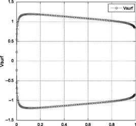
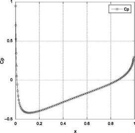
Calculate the pressure coefficient over an NACA0012 aerofoil with the source panel method, where the freestream attack angle is zero. Show the aerofoil shape, list the code for this, plot the source strength vari­ation, tangential flow speed distribution over the aerofoil surface and the pressure coefficient distribution over the aerofoil.

Solution

NACA0012 profile used is shown in Figure 7.10.

The FORTRAN program to calculate the pressure distribution over an aerofoil is given below:

c source panel method

c

program spm c

integer dim parameter (dim=200) c

c*****Variables

c	num	number of panels
c	(xn, yn)	nodes
c	(xc, yc)	control points (mid-point of control points	(i) and (i+1
c	phi	panel angle
c	s	panel length
c	SS	source strength (referenced as lambda in the	main text)
c	P, Q	matrics and vectors s. t. [P][SS]=[Q]
c	Vinf	free-stream velocity
c	Vsurf	flow speed at control point
c c c c	Cp	pressure coeff.
indx :	vector that records the row permutation

dimension xn(dim)/yn(dim)/xc(dim)/yc(dim)/phi(dim)/s(dim)

dimension P(dim/dim)/Q(dim)/SS(dim) dimension Vc(dim/dim)/Vsurf(dim)/Cp(dim) dimension indx(dim)

c pi=3.14………

pi = 4.0*atan(1.0) c

Vinf = 1.0 c

c******** input nodes over the surface

open(unit=50,file=’naca0012.txt’,form=’formatted’) read(50,*) num do 100 i=1,num

read(50,*) xn(i),yn(i)

100 continue c num = 8

c do 100 i=1,num

c xn(i) = cos( (180.+22.5-45.0*float(i-1))*pi/180. )

c yn(i) = sin( (180.+22.5-45.0*float(i-1))*pi/180. )

c 100 continue c

c Add an extra point to wrap back around to beginning

xn(num+1) = xn(1) yn(num+1) = yn(1) close(unit=50) c

c******** Calculate constants on each panel do 200 i=1,num

c – Set panel midpoint as control point

xc(i) = ( xn(i) + xn(i+1) ) /2.0 yc(i) = ( yn(i) + yn(i+1) ) /2.0 c – Panel length

s(i) = sqrt( (xn(i+1) – xn(i))**2 + (yn(i+1) – yn(i))**2 ) c – Panel angle

phi(i) = acos((xn(i+1) – xn(i)) / s(i)) if(yn(i+1).lt. yn(i)) phi(i)=2.0*pi-phi(i) c – Calc. vector Q

Q(i) = Vinf*sin(phi(i))

200 continue c

c******** Calculate components of matrix P do 300 j=1,num do 300 i=1,num

if (i. ne. j) then

	– aa, bb, ..	. are referenced as A,	B, …	in the main text.
	aa =
&	(-(xc(i)	– xn(j)	)*cos(phi(j)) –	(yc(i)	– yn(j))*sin(phi(j)
	bb = (xc(i) – xn(j))**2 + (yc(i)	– yn(j	))**2
	cc = sin(phi(i)	– phi(j))
	dd =
&	(yc(i)	– yn(j	))*cos(phi(i)) –	– (xc(i)	– xn(j))*sin(phi(i
	ee =
&	(xc(i)	– xn(j	))*sin(phi(j)) –	– (yc(i)	– yn(j))*cos(phi(j
	P(i, j) =	(cc/2.)	*log((s(j)**2+2.	.*aa*s(j	)+bb)/bb)

+ (dd-aa*cc)/ee*(atan((s(j)+aa)/ee)-atan(aa/ee))

&

P(i, j) =P(i, j) / (2.0*pi)

Vc(i, j)=(dd-aa*cc)/(2.0*ee)*log((s(j)**2+2.0*aa*s(j)+bb)/bb) & – cc*(atan((s(j)+aa)/ee) – atan(aa/ee))

else

P(i, j) = 1.0/2.0 Vc(i, j)= 0.0 end if

300 continue c

c******** Find SS by solving P. SS=Q

c with LU decomposition and back-substitution

call LUdcmp(P/num/indx/d) call LUbksb(P/num/indx/Q) do 350 i=1,num SS(i) = Q(i)

350 continue c

c********Calc. Pressure coeff. do 400 i=1,num

Vsurf(i) = Vinf*cos(phi(i)) do 410 j=1,num

if (i. ne. j) Vsurf(i) = Vsurf(i) + SS(j)/(2.0*pi)*Vc(i, j) 410 continue

Cp(i) = 1.0 – (Vsurf(i)/Vinf)**2 400 continue c

c******** Results

open(unit=51,file=’result. txt’,form=’formatted’) write(51,*) ‘x y Cp SourceStrength Vsurf’ c write( 6,*) ‘x y Cp SourceStrength Vsurf’

write( 6,*) ‘x phi[deg] Cp SourceStrength/2piV Vsurf’ do 500 i=1,num

write(51,550) xc(i),yc(i),Cp(i),SS(i),Vsurf(i) c write( 6,550) xc(i),yc(i),Cp(i),SS(i),Vsurf(i)

write( 6,550) xc(i),phi(i)*180/pi, Cp(i),SS(i)/(2.*pi*Vinf)

& ,Vsurf(i)

500 continue

550 format(‘ ‘,E15.8,’ ‘,E15.8,’ ‘,E15.8,’ ‘,E15.8,’ ‘,E15.8)

stop end c c

c================================================================

c******** Subroutines

subroutine LUdcmp(a, n,indx, d) parameter(dim=200,epsln=1.0e-20) dimension indx(dim),a(dim, dim),vv(dim) c

d=1.0

c

do 100 i=1,n aamax=0.0 do 110 j=1,n

if (abs(a(i, j)) .gt. aamax) aamax = abs(a(i, j))

110 100 c 220 210 240	continue if (aamax. eq.0.) then write(6,*) ‘singular matrix in LUdcmp’ pause end if vv(i) = 1.0 / aamax continue do 200 j = 1,n do 210 i=1,j-1 sum = a(i, j) do 220 k=1,i-1 sum=sum-a(i, k)*a(k, j) continue a(i, j) = sum continue aamax = 0.0 do 230 i=j, n sum = a(i, j) do 240 k=1,j-1 sum = sum – a(i, k) *a(k, j) continue a(i, j) = sum dum = vv(i) * abs(sum) if (dum. ge. aamax) then imax = i aamax = dum endif continue if (j. ne. imax) then do 250 k=1,n dum = a(imax, k) a(imax, k) = a(j, k) a(j, k) = dum continue d = – d vv(imax) = vv(j) endif indx(j) = imax if(a(i, j) .eq. 0.0) a(i, j) = epsln if(j. ne. n) then dum = 1.0 / a(j, j) do 260 i=j+1,n a(i, j) = a(i, j)*dum continue endif continue return end
230 250
260 200 c c
subroutine LUbksb(a/n/indx/b) parameter(dim=200) dimension indx(dim)/a(dim/dim)/b(dim)

c

ii = 0

do 100 i=1,n

ll = indx(i) sum = b(ll) b(ll)= b(i) if (ii. ne. 0) then do 110 j=ii, i-1

sum = sum – a(i, j)*b(j) 110 continue

else if (sum. ne. 0.0) then ii = i endif

b(i) = sum 100 continue

do 200 i=n,1,-1 sum = b(i) do 210 j=i+1,N

sum = sum – a(i, j)*b(j)

210 continue

b(i) = sum / a(i, i)

200 continue return end c

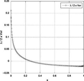
The source strength over the aerofoil surface is plotted in Figure 7.11. The tangential speed variation is shown in Figure 7.12.

The Cp distribution over the aerofoil is shown in Figure 7.13.

Figure 7.11 Source strength over the aerofoil.

x Figure 7.12 Tangential speed variation over the aerofoil.

Figure 7.13 The Cp distribution over the aerofoil.

Example 7.3

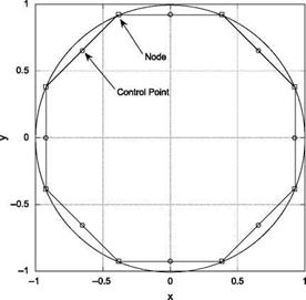
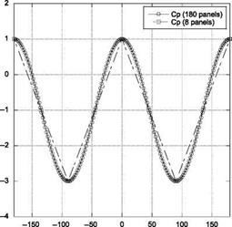
Calculate the pressure coefficient over a cylinder with unit diameter using the source panel method. List the program, compute and compare the pressure coefficient variation over the cylinder, representing it with 8 panels and with 180 panels. Also, show the source strength variation over the cylinder front to rear end.

Solution

The program in FORTRAN is given below.

c source panel method

c

program spm c

implicit none

parameter, integer (dim=200) c

c*****Variables

c	num	number of panels
c	(xn, yn)	nodes
c	(xc, yc)	control points (mid-point of control points	(i) and (i+1
c	phi	panel angle
c	s	panel length
c	SS	source strength (referenced as lambda in the	main text)
c	P, Q,SS	matrics and vectors s. t. [P][SS]=[Q]
c	Vinf :	free-stream velocity
c	Vsurf :	flow speed at control point
c c c c	Cp	pressure coeff.
indx :	vector that records the row permutation

real, dimension xn(dim),yn(dim),xc(dim),yc(dim),phi(dim),s(dim) real, dimension P(dim, dim),Q(dim),SS(dim) real, dimension Vc(dim, dim),Vsurf(dim),Cp(dim) integer, dimension indx(dim)

c pi=3.14………

pi = 4.0*atan(1.0) c

Vinf = 1.0 c

c******** input nodes over the surface num = 8

do 100 i=1,num

xn(i) = cos( (-22.5+45.0*float(i-1))*pi/180. ) yn(i) = sin( (-22.5+45.0*float(i-1))*pi/180. )

100 continue c

c Add an extra point to wrap back around to beginning

xn(num+1) = xn(1) yn(num+1) = yn(1) close(unit=50)

c c[12] c

c 200 c c****

300 c c****

c c**** 410 400 c c****

**** Calculate constants on each panel do 200 i=1,num

– Set panel midpoint as control point

xc(i) = ( xn(i) + xn(i+1) ) /2.0 yc(i) = ( yn(i) + yn(i+1) ) /2.0

– Panel length

s(i) = sqrt( (xn(i+1) – xn(i))**2 + (yn(i+1) – yn(i))**2 )

– Panel angle

phi(i) = asin((yn(i+1) – yn(i)) / s(i)) if(yn(i+1).lt. yn(i)) phi(i) = phi(i)+pi

– Calc. vector Q

Q(i) = – Vinf*sin(phi(i)) continue

**** Calculate components of matrix P do 300 j=1,num do 300 i=1,num

if (i. ne. j) then

– aa, bb, … are referenced as A, B, … in the main text. aa =

& (-(xc(i) – xn(j))*cos(phi(j)) – (yc(i) – yn(j))*sin(phi(j)))

bb = (xc(i) – xn(j))**2 + (yc(i) – yn(j))**2 cc = sin(phi(i) – phi(j))

&	dd = (yc(i)	1 – yn(j))*cos(phi(i)) – (xc(i)	– xn(j))	*sin(phi(i
&	ee = (xc(i)	1 – xn(j))*sin(phi(j)) – (yc(i)	– yn(j))	*cos(phi(j
&	P(i, j) = +	(cc/2.)*log((s(j)**2+2.*aa*s(j)+bb)/bb) (dd-aa*cc)/ee*(atan((s(j)+aa)/ee)-atan(aa/ee))
	P(i, j) =	P(i, j) / (2.0*pi)

Vc(i, j)=(dd-aa*cc)/(2.0*ee)*log((s(j)**2+2.0*aa*s(j)+bb)/bb)

& – cc*(atan((s(j)+aa)/ee) – atan(aa/ee))

else

P(i, j) = 1.0/2.0

Vc(i, j)= 0.0 end if continue

**** Find SS by solving P. SS=Q with LU decomposition call LUdcmp(P, num, indx, d) call LUbksb(P, num, indx, Q)

****Calc. Pressure coeff. do 400 i=1,num SS(i) = Q(i)

Vsurf(i) = Vinf*cos(phi(i)) do 410 j=1,num

if (i. ne. j) Vsurf(i) = Vsurf(i) + SS(i)/(2.0*pi)*Vc(i, j) continue

Cp(i) = 1.0 – (Vsurf(i)/Vinf)**2 continue

open(unit=51,file=’result. txt’,form=’formatted’) write(51,*) ‘x y Cp SourceStrength Vsurf’ write( 6,*) ‘x phi Cp SourceStrength Vsurf’ do 500 i=1,num

write(51,550) xc(i),yc(i),Cp(i),SS(i),Vsurf(i) write( 6,550) xc(i),phi(i)*180/pi, Cp(i),SS(i),Vsurf(i) 500 continue

550 format(‘ ‘,E15.8,’ ‘,E15.8,’ ‘,E15.8,’ ‘,E15.8,’ ‘,E15.8) stop end

c==============================================================

c******** Subroutines

subroutine LUdcmp(a, n,indx, d) parameter(dim=200,epsln=1.0e-20) dimension indx(dim),a(dim, dim),vv(dim) c

d=1.0

c

do 100 i=1,n aamax=0.0 do 110 j=1,n

if (abs(a(i, j)) .gt. aamax) aamax = abs(a(i, j))

110 continue

if (aamax. eq.0.) then

write(6,*) ‘singular matrix in LUdcmp’ pause end if

vv(i) = 1.0 / aamax 100 continue c

do 200 j=1,n

do 210 i=1,j-1 sum = a(i, j) do 220 k=1,i-1

sum=sum-a(i, k)*a(k, j)

220 continue

a(i, j) = sum 210 continue

aamax = 0.0 do 230 i=j, n sum = a(i, j) do 240 k=1,j-1

sum = sum – a(i, k) *a(k, j)

240 continue

a(i, j) = sum dum = vv(i) * abs(sum) if (dum. ge. aamax) then imax = i aamax = dum endif

230 continue

if (j. ne. imax) then do 250 k=1,n

dum = a(imax, k)

a(imax, k) = a(j, k) a(j, k) = dum 250 continue

d = – d

vv(imax) = vv(j) endif

indx(j) = imax

if(a(i, j) .eq. 0.0) a(i, j) = epsln if(j. ne. n) then

dum = 1.0 / a(j, j) do 260 i=j+1,n

a(i, j) = a(i, j)*dum 260 continue

endif 200 continue return end c

subroutine LUbksb(a/n/indx/b) parameter(dim=200)

dimension indx(dim)/a(dim/dim)/b(dim) c

ii = 0

do 100 i=1,n

ll = indx(i) sum = b(ll) b(ll)= b(i) if (ii. ne. 0) then do 110 j=ii, i-1

sum = sum – a(i, j)*b(j)

110 continue

else if (sum. ne. 0.0) then ii = i endif

b(i) = sum 100 continue

do 200 i=n,1,-1 sum = b(i) do 210 j=i+1,N

sum = sum – a(i, j)*b(j)

210 continue

b(i) = sum / a(i, i)

200 continue return end c

Schematic of the cylinder with 8 panels is shown in Figure 7.14.

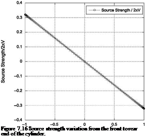
Nondimensional pressure distribution over the cylinder, computed with 8 panels and 180 panels are compared in Figure 7.15. Variation of source strength from the front end to the rear end of the cylinder is shown in Figure 7.16.

Figure 7.14 Cylinder with 8 panels.

Angle [deg] Figure 7.15 Variation of pressure coefficient over the cylinder.

x

Example 7.4

Write and list the code for solving flow past a NACA0012 aerofoil, using vortex panel method. Compute and plot lift and drag coefficients and the aerodynamic efficiency for angle of attack range from — 5° to +20°.

Solution

The FORTRAN program for vortex panel method is listed below:

matrics and vectors s. t. [P][gamma]=[Q]

free-stream velocity

angle of attack

flow speed at control point

pressure coeff.

vector that records the row permutation

dimension xn(dim)/yn(dim)/xc(dim)/yc(dim)/phi(dim)/s(dim) dimension P(dim/dim)/Q(dim)/gamma(dim) dimension Vsurf(dim),Cp(dim) dimension indx(dim)

dimension a(dim/dim)/b(dim/dim)/r(dim/dim)

pi=3.14….

pi = 4.0*atan(1.0)

c

c – free-stream speed Vinf = 1.0

c – angle of attack (deg.) alpha = 8.0

alpha = alpha * pi/180.

c

c******** input nodes over the surface

open(unit=50,file=’naca0012.txt’,form=’formatted’) read(50,*) num do 100 i=1,num

read(50,*) xn(i),yn(i)

100 continue

c Add an extra point to wrap back around to beginning

xn(num+1) = xn(1) yn(num+1) = yn(1) close(unit=50)

c

c******** Calculate constants on each panel do 200 i=1,num

c – Set panel midpoint as control point

xc(i) = ( xn(i) + xn(i+1) ) /2.0 yc(i) = ( yn(i) + yn(i+1) ) /2.0 c – Panel length

s(i) = sqrt( (xn(i+1) – xn(i))**2 + (yn(i+1) – yn(i))**2 ) c – Panel angle

phi(i) = acos((xn(i+1) – xn(i)) / s(i)) if(yn(i+1).lt. yn(i)) phi(i)=2.0*pi-phi(i) c – Calc. vector Q

Q(i) = Vinf*sin(alpha – phi(i))

200 continue

Q(num+1) = 0.0

c

c******** Calculate components of matrix P do 300 j=1,num+1 do 300 i=1,num

r(i, j) = sqrt( (xc(i)-xn(j))**2 + (yc(i)-yn(j))**2 ) 300 continue

do 310 j=1,num

do 310 i=1,num

xcl = (xc(i)-xn(j))*cos(phi(j)) + (yc(i)-yn(j))*sin(phi(j)) ycl =-(xc(i)-xn(j))*sin(phi(j)) + (yc(i)-yn(j))*cos(phi(j))

340 c c[13] c

350 c c****

beta= atan(xcl/ycl) – atan((xcl-s(j))/ycl)

cc = (1./(2.*pi))*(-(1.-xcl/s(j))*log(r(i, j+1)/r(i, j))

& + (1.-ycl/s(j)*beta) )

dd = (1./(2.*pi))*( (1.-xcl/s(j))*beta & – ycl/s(j)*log(r(i, j+1)/r(i, j)) )

ee = (1./(2.*pi))*(-xcl/s(j)*log(r(i, j+1)/r(i, j))

& – (1.-ycl/s(j)*beta) )

ff = (1./(2.*pi))*( xcl/s(j)*beta

& + ycl/s(j)*log(r(i, j+1)/r(i, j)) )

a(i, j) = cc*cos(phi(i)-phi(j)) + dd*sin(phi(i)-phi(j)) b(i, j) = ee*cos(phi(i)-phi(j)) + ff*sin(phi(i)-phi(j)) continue do 320 i=1,num do 330 j=2,num

P(i, j) = a(i, j) + b(i, j-1) continue j=1

P(i,1) = a(i,1)

j=num+1

P(i, num+1)= b(i, num) continue

do 340 j=1,num+1 P(num+1,j) = 0.

if(j. eq.1.or. j.eq. num+1) P(num+1,j)=1. continue

**** Find SS by solving P. SS=Q

with LU decomposition and back-substitution call LUdcmp(P/num+1/indx/d) call LUbksb(P/num+1/indx/Q) do 350 i=1,num+1 gamma(i) = Q(i) continue

2 *log(r(i, j+1)/r(i, j))

3 + (1.0/(2.*pi))*(gamma(j+1)-gamma(j))*(1.-ycl/s(j)*beta)

dphi = phi(i)-phi(j)

Vsurf(i) = Vsurf(i) + ulocal*cos(dphi)+vlocal*sin(dphi) endif

410 continue

Cp(i) = 1.0 – (Vsurf(i)/Vinf)**2 400 continue

c

c******** Results

open(unit=51,file=’result. txt’,form=’formatted’) write(51,*) ‘x y Cp Vortex Vsurf’ write( 6,*) ‘x phi[deg] Cp Vortex Vsurf’ do 500 i=1,num

gam=(gamma(i)+gamma(i+1))/2.

write(51,550) xc(i),yc(i),Cp(i),gam, Vsurf(i)

write( 6,550) xc(i),phi(i)*180/pi, Cp(i),gam, Vsurf(i)

500 continue

550 format(‘ ‘,E15.8,’ ‘,E15.8,’ ‘,E15.8,’ ‘,E15.8,’ ‘,E15.8)

c

c******** Lift and Drag Coefficients & L/D Cx = 0.0 Cy = 0.0 do 560 i=1,num

Cx = Cx + (yn(i+1)-yn(i))*Cp(i)

Cy = Cy – (xn(i+1)-xn(i))*Cp(i)

560 continue

Cl =-Cx*sin(alpha) + Cy*cos(alpha)

Cd = Cx*cos(alpha) + Cy*sin(alpha)

write(6,*) ‘======== Aerodynamic Coefficients ========’

write(6,*) ‘Lift Coeff. = ‘,Cl write(6,*) ‘Drag Coeff. = ‘,Cd write(6,*) ‘ L/D = ‘,Cl/Cd

write(6,*) ‘==========================================’

stop

end

c=============================================================

c******** Subroutines

subroutine LUdcmp(a, n,indx, d) integer dim

parameter(dim=200,epsln=1.0e-20) dimension indx(dim),a(dim, dim),vv(dim)

c

d=1.0

c

do 100 i=1,n aamax=0.0 do 110 j=1,n

if (abs(a(i, j)) .gt. aamax) aamax = abs(a(i, j))

110 continue

if (aamax. eq.0.) then

write(6,*) ‘singular matrix in LUdcmp’ pause end if

vv(i) = 1.0 / aamax continue do 200 j = 1,n do 210 i=1,j-1 sum = a(i, j) do 220 k=1,i-1 sum=sum-a(i/k)*a(k/j) continue a(i, j) = sum continue aamax = 0.0 do 230 i=j, n sum = a(i, j) do 240 k=1,j-1 sum = sum – a(i, k) *a(k, j) continue a(i, j) = sum dum = vv(i) * abs(sum) if (dum .ge. aamax) then imax = i aamax = dum endif continue if (j. ne. imax) then do 250 k=1,n dum = a(imax, k) a(imax, k) = a(j, k) a(j, k) = dum continue d = – d vv(imax) = vv(j) endif indx(j) = imax if(a(i, j) .eq. 0.0) a(i, j) = epsln if(j. ne. n) then dum = 1.0 / a(j, j) do 260 i=j+1,n a(i, j) = a(i, j)*dum continue endif continue return end subroutine LUbksb(a/n/indx/b) integer dim parameter(dim=200) dimension indx(dim)/a(dim/dim)/b(dim) ii = 0 do 100 i=1,n ll = indx(i) = b(ll)

100 c 220 210 240

230 250

260 200 c c

sum

b(ll)= b(i) if (ii. ne. 0) then do 110 j=ii, i-1

sum = sum – a(i, j)*b(j) 110 continue

else if (sum. ne. 0.0) then ii = i endif

b(i) = sum 100 continue

do 200 i=n,1,-1 sum = b(i) do 210 j=i+1,N

sum = sum – a(i, j)*b(j)

210 continue

b(i) = sum / a(i, i)

200 continue return end

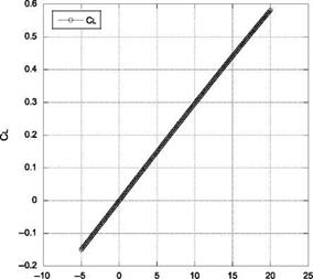
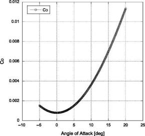
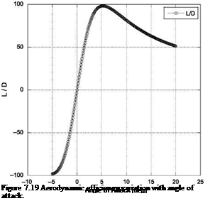
The lift and drag coefficient variation with the angle of attack for NACA0012 aerofoil, computed by vortex panel method, are shown in Figures 7.17 and 7.18, respectively. Variation of the aerodynamic efficiency of the aerofoil, calculated from the lift and drag computed with the vortex panel method, is shown in Figure 7.19.

Angle of Attack [deg] Figure 7.17 Lift coefficient variation with angle of attack.

Figure 7.18 Drag coefficient variation with angle of attack.

7.3 Summary

Panel method is a numerical technique to solve flow past bodies by replacing the body with mathematical models; consisting of source or vortex panels. These are referred to as source panel and vortex panel methods, respectively.

In general, the source strength X(s) can change from positive (+ve) to negative (—ve) along the source sheet. That is, the “source” sheet can be a combination of line sources and line sinks.

The velocity potential at point P due to all the panels can be obtained by taking the summation of the above equation over all the panels. That is:

n

ф(р) = J2 Аф = J2 ln rpjds

where the distance:

rpj = J(x – Xj)2 + (y – yj)2,

where (xj, yj) are the coordinates along the surface of the jth panel.

The boundary condition is at the control points on the panels and the normal component of flow velocity is zero.

The boundary condition states that:

Vi, n + Vn =

Therefore:

n Vn = 1 + £ 2n	dn (ln rij) dsj + Vi cos в = 0
j=1,j = i	‘j 1

This is the heart of source panel method. The values of the integral in this equation depend simply on the panel geometry, which are not the properties of the flow.

Once source strength distributions k1 are obtained, the velocity tangential to the surface at each control point can be calculated. The pressure coefficient Cp at the ith control point is:

For compressible flows the pressure coefficient becomes:

The vortex panel method is analogous to the source panel method studied earlier. The source panel method is useful only for nonlifting cases since a source has zero circulation associated with it. But vortices have circulation, and hence vortex panels can be used for lifting cases. It is once again essential to note that the vortices distributed on the panels of this numerical method are essentially free vortices.

Therefore, as in the case of source panel method, this method is also based on a fundamental solution of the Laplace equation. Thus this method is valid only for potential flows which are incompressible.

• The mid-point of each panel is a control point at which the boundary condition is applied; that is, at each control point, the normal component of flow velocity is zero.

This equation is the crux of the vortex panel method. The values of the integrals in this equation depend simply on the panel geometry; they are properties of the flow.

Pressure distribution around a body, given by source panel method is:

This is the general expression for two arbitrarily oriented panels; it is not restricted to circular cylinder only.

Exercise Problems

1. Using vortex panel method, compute and plot (a) the pressure coefficient distribution over a NACA0012 aerofoil and (b) the variation of drag coefficient with lift coefficient, for — in the range from -0.15 to 0.55, if the aerofoil is at an angle of attack of 8° in a uniform freestream.

2. List the procedure steps, along with equations, involved in the FORTRAN code vortex panel method given in Example 7.4.

3. Compute and plot the pressure coefficient variation over a NACA0012 aerofoil in a uniform freestream at angles of attack 0, 2, 5 and 8 degrees. Also plot the vortex distribution over the aerofoil profile for these angles.

Reference

1. Magnus, A. E., and Epton, M. A., “PAN AIR – A computer program for predicting subsonic or supersonic linear potential flows about arbitrary configurations using a higher order panel method”, Volume I – Theory Document (Version 1.0), NASA CR 3251, April 1980.

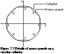
Let us consider a circular cylinder with a distribution of source panels on its circumference, as shown in Figure 7.7.

To evaluate the integral Ij, let us consider the ith and jth panels, as illustrated in Figure 7.8.

The control point on the ith panel is (x;, y;). Coordinates of boundary points of ith panel are (x;, y;) and (x;+1, y;+i). An elemental length segment dsj on the jth panel is at a distance of r;j from (x;, y;), as shown in Figure 7.8. The point (xj, yj) is the running point on the jth panel. The boundary points of the

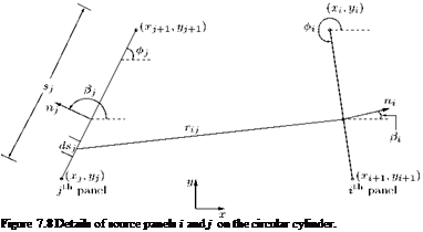Vcc