Category THEORETICAL AERODYNAMICS

This method is analogous to the source panel method studied earlier. The source panel method is useful only for nonlifting cases since a source has zero circulation associated with it. But vortices have circu­lation, and hence vortex panels can be used for lifting cases. It is once again essential to note that the vortices distributed on the panels of this numerical method are essentially free vortices. Therefore, as in the case of source panel method, this method is also based on a fundamental solution of the Laplace equation. Thus this method is valid only for potential flows which are incompressible.

7.3.1 Application of Vortex Panel Method

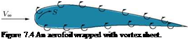
Consider the surface of an aerofoil wrapped with vortex sheet, as shown in Figure 7.4.

We wish to find the vortex distribution y (s) such that the body surface becomes a streamline of the flow. There exists no closed-form analytical solution for y(s); rather, the solution must be obtained numerically. This is the purpose of the vortex panel method.

The procedure for obtaining solution using vortex panel method is the following: [10]

• The mid-point of each panel is a control point at which the boundary condition is applied; that is, at each control point, the normal component of flow velocity is zero.

Let P be a point located at (x, y) in the flow, and let rpj be the distance from any point on the jth panel to P. The radial distance rPj makes an angle 0pj with respect to x-axis. The velocity potential induced at P due to the jth panel [Equation (2.42)] is:

=~2L jj^j

The component of velocity normal to the ith panel is given by:

VX, n VX cos fti.

The normal component of velocity induced at (xi, yi) by the vortex panels is:

d

Vn – dn ^ *>]. (7Л3)

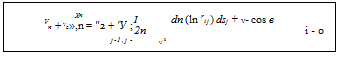
From Equations (7.11) and (7.13), we get the normal component of velocity induced as:

By the boundary conditions, at the control point of the ith, we have:

Vix>,n + Vn — ^

that is:

(7.16)

This equation is the crux of the vortex panel method. The values of the integrals in Equation (7.16) depend simply on the panel geometry; they are properties of the flow.

Let Jj be the value of this integral when the control point is on the ith panel. Now, Equation (7.16) can be written as:

n

Vx cos в – у jjj — 0. (7.17)

j—1

Equation (7.17) is a linear algebraic equation with n unknowns, y,yi, y3, …., yn. It represents the flow boundary conditions evaluated at the control point of the jth panel. If Equation (7.13) is applied to the control points of all the panels, we obtain a system of n linear equations with n unknowns.

The discussion so far has been similar to that of the source panel method. For source panel method, the n equations for the n unknown source strength are routinely solved, giving the flow over a nonlifting body.

For a lifting body with vortex panels, in addition to the n equations given by Equation (7.17) applied at all the panels, we must also ensure that the Kutta condition is satisfied. This can be done in many ways. For example, consider the trailing edge of an aerofoil, as shown in Figure 7.5, illustrating the details of vortex panel distribution at the trailing edge.

Note that the length of each panel can be different, their length and distribution over the body is at our discretion. Let the two panels at the trailing edge be very small. The Kutta condition is applied at the trailing edge and is given by:

Y (te) = 0.

To approximate this numerically, if points i and (i — 1) are close enough to the trailing edge, we can write:

Yi = Yi— 1. (7.18)

such that the strength of the two vortex panels i and (i — 1) exactly cancel at the point where they touch at the trailing edge. Thus, the Kutta condition demands that Equation (7.18) must be satisfied.

Note that Equation (7.17) is evaluated at all the panels and Equation (7.18) constitutes an over­determined system of n unknowns with (n + 1) equations. Therefore, to obtain a determined system, Equation (7.17) is evaluated at one of the control points. That is, we choose to ignore one of the control points, and evaluate Equation (7.17) at the other (n — 1) control points. This, on combination with Equation (7.18), gives n linear algebraic equations with n unknowns.

At this state, conceptually we have obtained Yi, Y2, Y3,……… ,Yn which make the body surface a stream­

line of the flow and which also satisfy the Kutta condition. In turn, the flow velocity tangential to the
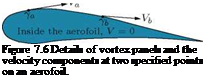
surface can be obtained directly from y. To see this more clearly, consider the aerofoil shown in Figure 7.6.
The velocity just inside the vortex sheet on the surface is zero. This corresponds to u2 = 0. Hence:

Y = U1 — U2 = U1 — 0 = U1.

Therefore, the local velocities tangential to the aerofoil surface are equal to the local values of Y. In turn the local pressure distribution can be obtained from Bernoulli’s equation. The total circulation around the aerofoil is:

n

Г = £) Yjj. (7.19)

j=1

Flow

Hence, the lift per unit span is:

Once source strength distributions Xi are obtained, the velocity tangential to the surface at each control point can be calculated as follows.

Let s be the distance along the body surface, as shown in Figure 7.3, measured positive (+ve) from front to rear. The component of freestream velocity tangential to the surface is:

Vc»,s V(X> sin Pi.

The tangential velocity Vs at the control point of the ith panel induced by all the panels is obtained by differentiating Equation (7.1) with respect to s. That is:

Note that the tangential velocity Vs on a flat source panel induced by the panel itself is zero; hence in Equation (7.6), the term corresponding to j = i is zero. This is easily seen by intuition, because the panel can emit volume flow only in a direction perpendicular to its surface and not in the direction tangential to its surface.

The surface velocity Vi at the control point of the ith panel is the sum of the contribution V, x,s from the freestream and Vs given by Equation (7.6).

The pressure coefficient Cp at the ith control point is:

(7.8)

Note: It is important to note that the pressure coefficient given by Equation (7.8) is valid only for incompressible flows with freestream Mach number less than 0.3. For compressible flows the pressure coefficient becomes:

where pi is the static pressure at the ith panel and px, px and Vx, respectively, are the pressure, density and velocity of the freestream flow. The dynamic pressure can be expressed as:

Dividing the numerator and denominator of the right-hand side by y, we have the dynamic pressure as:

yp x Vx

2 aL, ’

since aI = yRTx. This simplifies to:

2 PxV2 = Y2x mi.

Thus the pressure coefficient for compressible flows becomes:

7.2.1.1 Test on Accuracy

Let Sj be the length of the /h panel and Xj be the source strength of the /h panel per unit length. Hence, the strength of the jth panel is XjSj. For a closed body, the sum of the strengths of all the sources and sinks must of zero, or else the body itself would be adding or absorbing mass from the flow. Hence, the values of the Xjs obtained above should obey the relation:

This equation provides an independent check on the accuracy of the numerical results.

7.1 Introduction

Panel method is a numerical technique to solve flow past bodies by replacing the body with mathematical models; consisting of source or vortex panels. Essentially the surface of body to be studied will be represented by panels consisting of sources and free vortices. These are referred to as source panel and vortex panel methods, respectively. If the body is a lift generating geometry, such as an aircraft wing, vortex panel method will be appropriate for solving the flow past, since the lift generated is a function of the circulation or the vorticity around the wing. If the body is a nonlifting structure such as a pillar of a river bridge, the source panel method might be employed for solving the flow past that.

7.2 Source Panel Method

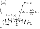
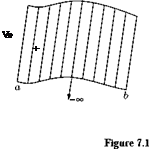
Consider the source sheet of finite length along the ^-direction and extending to infinity in the direction normal to s, as shown in Figure 7.1.

The source strength per unit length along s-direction of the panel, shown in Figure 7.1, is X = X(s). Also, the small length segment ds is treated as a distinct source of strength X ds.

Let us consider a point P as shown in Figure 7.1. The small segment of the source sheet of strength X ds induces an infinitesimally small velocity potential dф at point P. That is:

X ds

= —– ln r.

2n

The complete velocity potential at point P, due to source sheet from a to b, is given by:

In general, the source strength X(s) can change from positive (+ve) to negative (—ve) along the source sheet. That is, the ‘source’ sheet can be a combination of line sources and line sinks.

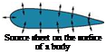
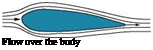
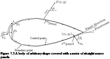
Next, let us consider a given body of arbitrary shape shown in Figure 7.2.

Let us assume that the body surface is covered with a source sheet, as shown in Figure 7.2(a), where the strength of the source X (s) varies in such a manner that the combined action of the uniform flow and the source sheet makes the aerofoil surface and streamlines of the flow, as shown in Figure 7.2(b).

Theoretical Aerodynamics, First Edition. Ethirajan Rathakrishnan.

© 2013 John Wiley & Sons Singapore Pte. Ltd. Published 2013 by John Wiley & Sons Singapore Pte. Ltd.

Uniform

flow

Figure 7.2 An arbitrary body (a) covered with source sheet, (b) the flow past it.

The problem now becomes that of finding appropriate distribution of k(y), over the surface of the body.

The solution to this problem is carried out numerically, as follows:

• Approximate the source sheet by a series of straight panels, as shown in Figure 7.3.

• Let the source strength k(y) per unit length be constant over a given general panel, but allow it to vary

from one panel to another. That is, for n panels the source strengths are k, k2, k3,………. , kn.

• The main objective of the panel technique is to solve for the unknowns kj, j = 1 to n, such that the body surface becomes a stream surface of the flow.

•

This boundary condition is imposed numerically by defining the mid-point of each panel to be a control point and by determining the kjs such that the normal component of the flow velocity is zero at each point.

Let P be a point at (x, y) in the flow, and let rpj be the distance from any point on the /h panel to point P, as shown in Figure 7.3. The velocity at P due to the /h panel, Афj, is:

Афі = 2П Iln rPjdsj,

where the source strength Xj is constant over the jth panel, and the integration is over the jth panel only.

The velocity potential at point P due to all the panels can be obtained by taking the summation of the above equation over all the panels. That is:

ф(р) = ^ Аф = ^2 2n Iln rpjds

j=i

where the distance:

rPj = J(x – xj)2 + (y – yj)2,

where (xj, yj) are the coordinates along the surface of the jth panel.

Since P is just an arbitrary point in the flow, it can be taken at anywhere in the flow including the surface of the body, which can be regarded as a stream surface (essentially the stagnation stream surface). Let P be at the control point of the ith panel. Let the coordinates of this control point be given by (x;, y;), as shown in Figure 7.3. Then:

(7.1)

where

rij = J (xi – xj)2 + (y; – yj)2.

Equation (7.1) is physically the contribution of all the panels to the potential at the control point on the ith panel.

The boundary condition is at the control points on the panels and the normal component of flow velocity is zero. Let n be the unit vector normal to the ith panel, directed out of the body.

The slope of the ith panel is (dy/dx);. The normal component of velocity with respect to the ith panel is:

V^,n V(X> ‘ ni V(X> cos Pi,

where в; is the angle between VOT and n;. Note that Vai, n is positive (+ve) when directed away from the body.

The normal component of velocity induced at (x;, y;) by the source panel, from Equation (7.1), is:

When the differentiation in Equation (7.2) is carried out, rij appears in the denominator. Therefore, a singular point arises on the ith panel because at the control point of the panel, j = i and rtj = 0. It can be

shown that when j – i, the contribution to the derivative is X/2. Therefore:

where Xi/2 is the normal velocity induced at the ith control point by the ith panel itself.

The normal component of flow velocity is the sum of the normal components of freestream velocity V—,n and velocity due to the source panel Vn. The boundary condition states that:

V _i_ V — 0

Therefore, the sum of Equation (7.3) and V—,n results in:

(7.4)

This is the heart of source panel method. The values of the integral in Equation (7.4) depend simply on the panel geometry, which are not the properties of the flow.

Let I-j be the value of this integral when the control point is on the ith panel and the integral is over the jth panel. Then, Equation (7.4) can be written as:

This is a linear algebraic equation with n unknowns Л1, X2, ………… , Xn. It represents the flow boundary

condition evaluated at the control point of the ith panel.

Now let us apply the boundary condition to the control points of all the panels, that is, in Equation (7.5), let i — 1, 2, 3, …., n. The results will be a system of n linear algebraic equations with n unknowns (X1, X2, , Xn), which can be solved simultaneously by conventional numerical methods:

• After solving the system of equations represented by Equation (7.5) with i — 1, 2, 3, …., n, we have the distribution source panel strength which, in an approximate fashion, causes the body surface to be a streamline of the flow.

• This approximation can be made more accurate by increasing the number of panels, hence more closely representing the source sheet of continuously varying strength X (s).

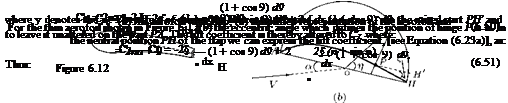
Let us consider an aerofoil whose rear part is movable about a hinge at P on the camber line, as shown in Figure 6.12(a). Essentially the rear part PH is the flap, which can be raised or lowered from the neutral position shown in the figure.

In an aerofoil of finite aspect ratio, the flap movement affects only part of a wing. Ailerons are flaps near the wing tips and are arranged so that the port and starboard ailerons move in opposite senses (that is, one up and one down). In our discussions here let us consider a two-dimensional problem for simplicity and assume that the aerofoil is thin, and the portion PH of the camber line is straight, and the angle § through which the flap is rotated is small.

Thus the effect of raising the flap is to decrease the lift coefficient, the effect of lowering the flap is to increase the lift coefficient. Therefore, in particular, when the flaps are lowered just before landing, increased lift is obtained (and also increased drag). In the case of ailerons, if the port aileron is raised and the starboard aileron depressed, the lift on the port wing is decreased and that on the starboard wing is increased, causing a rolling moment which tends to raise the starboard wing tip.

6.4 Summary

The overall lifting property of a two-dimensional aerofoil depends on the circulation it generates and this, for the far-field or overall effects, has been assumed to be concentrated at a point within the aerofoil profile, and to have a magnitude related to the incidence, camber and thickness of the aerofoil.

The loading on the aerofoil, or the chordwise pressure distribution, follows as a consequence of the parameters, namely the incidence, camber and thickness. But the camber and thickness imply a characteristic shape which depends in turn on the conformal transformation function and the basic flow to which it is applied.

The profiles obtained with Joukowski transformation do not lend themselves to modern aerofoil design. However, Joukowski transformation is of direct use in aerofoil design. It introduces some features which are the basis to any aerofoil theory, such as (a) the lift generated by an aerofoil is proportional to the circulation around the aerofoil profile, L а Г. (b) The magnitude of the circulation Г must be such that
it keeps the velocity finite in the vicinity of trailing edge. It is not necessary to concentrate the circulation in a single vortex, the vorticity can be distributed throughout the region surrounded by the aerofoil profile in such a way that the sum of the distributed vorticity equals that of the original model, and the vorticity at the trailing edge is zero. This mathematical model may be simplified by distributing the vortices on the camber line and disregarding the effect of thickness. In this form it becomes the basis for the classical “thin aerofoil theory” of Munk and Glauert.

The usefulness or advantage of the theory lies in the fact that the aerofoil characteristics could be quoted in terms of the coefficient Ax, which in turn could be found by graphical integration method from any camber line.

General thin aerofoil theory is based on the assumption the aerofoil is thin so that its shape is effectively that of its camber line and the camber line shape deviates only slightly from the chord line.

The camber line is replaced by a line of variable vorticity so that the total circulation about the chord is the sum of the vortex elements. Thus, the circulation around the camber becomes:

Г = f kSs.

J0

The lift per unit span is given by:

c

L = pUr = pU kdx.

0

Again for unit span, the moment of pressure forces about the leading edge is:

г г

Mle = — pxdx = —pU kx dx.

00

For a flat plate, dy/dx = 0. Therefore, the general equation [Equation (6.9)] simplifies to:

1 fc kdx

Ua =

The elementary circulation at any point on the flat plate is:

Lift per unit span is given by:

L = 1 pU2(c x 1)C

The lift coefficient CL becomes:

The pitching moment per unit span is:

—Mie = 2 pU2 c2a 1(—Cmu).

The pitching moment coefficient becomes:

For small values of angle of attack, a, the center of pressure coefficient, kcp, (defined as the ratio of the center of pressure from the leading edge of the chord to the length is chord), is given by:

This shows that the center of pressure, which is a fixed point, coincides with the aerodynamic center. This is true for any symmetrical aerofoil section.

The center of pressure is at the quarter-chord point for a symmetrical aerofoil.

By definition the point on the aerofoil where the moments are independent of angle of attack is called the aerodynamic center. The point from the leading edge of the aerofoil at which the resultant pressure acts is called the center of pressure. In other words, center of pressure is the point where line of action of the lift L meets the chord. Thus the position of the center of pressure depends on the particular choice of chord.

The center of pressure coefficient is defined as the ratio of the center of pressure from the leading edge of the aerofoil to the length of chord.

The moment about the quarter-chord point is zero for all values of a. Hence, for a symmetrical aerofoil, we have the theoretical result that “the quarter-chord point is both the center of pressure and the aerodynamic center.”

The aerodynamic center is located around the quarter chord point. Whereas the center of pressure is a moving point, strongly influenced by the angle of attack.

Center of pressure is the point at which the pressure distribution can be considered to act – analogous to the “center of gravity” as the point at which the force of gravity can be considered to act.

The horizontal position of the center of gravity has a great effect on the static stability of the wing, and hence, the static stability of the entire aircraft. If the center of gravity is sufficiently forward of the aerodynamic center, then the aircraft is statically stable. If the center of gravity of the aircraft is moved toward the tail sufficiently, there is a point – the neutral point – where the moment curve becomes horizontal; this aircraft is neutrally stable. If the center of gravity is moved farther back, the moment curve has positive slope, and the aircraft is longitudinally unstable.

For a circular arc aerofoil at an angle of attack a to the flow k can be expressed as:

The effect of camber is to increase k distribution by (2U x 2ft sin в) over that of the flat plate. Thus:

k — ka + kb,

where:

arises from the incidence of the aerofoil alone and:

which is due to the effect of the camber alone.

The lift L acting on the aerofoil can be expressed as:

L = I pU 2c 2n(a + 0)
Cl = 2п(а + в) •

Thus the lift-curve slope is:

From the above relations for Cl and dCL /da, it is evident that:

at a = 0, Cl = 2пв at a = —в, Cl = 0

and the lift-curve slope is independent of camber.

For a cambered aerofoil, we have:

2n (a + в)

dCL,

-da(a

For Cl = 0, a = —в or —aL=0 = в. Thus:

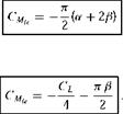
The pitching moment is:

Mie = —2pU2c2 ^(a + 2в) • Therefore, the pitching moment coefficient becomes:

or

The center of pressure coefficient, kcp, becomes:

Thus, the effect of camber is to set back the center of pressure by an amount which decreases with increasing incidence or lift.

The general camber line can be replaced by a chordwise distribution of circulation. That is:

k = ka + kb,

where

Note that this ka distribution satisfies the Kutta-Joukowski distribution, since ka = 0 when в = n, that is, at x = c.

The corresponding kb is represented by a Fourier series. Providing 0 < в < n, the end conditions are satisfied, and any variation in shape is accommodated if it is a sine series. Thus:

kb = 2U (Aj sin в + A2 sin 2в + A3 sin 3в + •• ••)

TO

= 2U ^ ‘ An sin пв.

1

Thus, k = ka + kb becomes:

The coefficients A0, A1, A2, • • ••, An can be obtained by substituting for k in the general equation (6.30), suitably converted with regard to units.

For a thin aerofoil, the circulation distribution is:

The lift is also given by:

1 2

L = – pU 2cCL.

Therefore, the lift coefficient becomes:

The pitching moment is given by:

-Mie = ~CMle-xPU c.

The pitching moment coefficient is:

The center of pressure coefficient is:

Flap at the trailing edge of an aerofoil is a high-lifting device, which when deflected down causes increase of lift, essentially by increasing the camber of the profile. The deflection of the flap about a hinge in the camber line effectively alters the camber of the profile so that the contribution due to flap deflection is an addition to the effect of camber line shape.

The chordwise circulation distribution due to flap deflection becomes:

The lift coefficient is:

CL = 2л a + 2(л — ф + sin ф) n.

Likewise, the pitching moment coefficient CMe is:

л l r, , 1

Cmu =—2 a — 2 П — ф + sin ф (2 — cos ф)] n.

The characteristic of a flapped aerofoil, which is of great importance in stability and control of the aircraft, is the aerodynamic moment about the hinge line, H:

H = Ch 2 pU 2(Fc)2.

In an aerofoil of finite aspect ratio, the flap movement affects only part of a wing. Ailerons are flaps near the wing tips and are arranged so that the port and starboard ailerons move in opposite senses (that is, one up and one down). The effect of raising the flap is to decrease the lift coefficient, the effect of lowering the flap is to increase the lift coefficient. Therefore, in particular, when the flaps are lowered just before landing, increased lift is obtained (and also increased drag). In the case of ailerons, if the port aileron is raised and the starboard aileron depressed, the lift on the port wing is decreased and that on the starboard wing is increased, causing a rolling moment which tends to raise the starboard wing tip.

Exercise Problems

1. Determine the maximum circulation due to camber of a circular arc aerofoil of percentage camber 0.05, in a flow of velocity 200 km/h.

[Answer: 0.2224 m2/s]

2. If the lift coefficient and lift curve slope of an aerofoil of percentage camber 0.6 are l.02 and 2, respectively, determine (a) the pitching moment about the leading edge and (b) the center ofpressure coefficient.

[Answer: (a) —0.254, (b) 0.2685]

3. If the elemental circulation at 30% chord of a flat plate in a flow at 40 m/s is 24 m2/s, determine the angle of attack.

[Answer: 11.25° ]

4. A two-dimensional wing of NACA 4412 profile flies at an incidence of 4°. Determine the lift coefficient of the wing.

[Answer: 1.024]

5. An aerofoil of average chord 1.2 m, at an angle of attack 2° to a flow at 45 m/s at sea level, experiences a lift of 500 N per unit area. Determine the pitching moment about the leading edge, (a) assuming the profile to be symmetrical and (b) assuming the profile is cambered with 3% camber.

[Answer: (a) -178.6 N-m, (b) -434 N-m]

6. A Joukowski profile of 3.3% camber is in an air stream of speed 60 m/s at an angle of attack of 4°. Determine the circulation around the maximum thickness location.

[Answer: 28.22 m2/s]

7. A parabolic camber line of unit chord length is at an incidence of 3° in a uniform flow of velocity 20 m/s. If the camber line is given by: determine the velocity induced at the mid-chord location, assuming the incidence as an ideal angle of attack.

[Answer: -3.14 m/s]

8. An aircraft of wing area 42 m2 and mean chord 3 m flies at 120 m/s at an altitude where the density is 0.905 kg/m3. The center of pressure is at 0.28 times mean chord behind the leading edge of the wing when the wing lift coefficient is 0.2. (a) If the lift on the tail plane acts through a point 8 m horizontally behind the center of pressure, determine the tail lift required to trim the aircraft. (b) Assuming the wing profile as a circular arc, find the percentage camber. Assume the pitching moments on the tail plane, fuselage and nacelles are negligibly small.

[Answer: (a) 5201 N, (b) 0.191]

9. A thin aerofoil of 3% camber in a freestream has a lift coefficient of 1.2. (a) If the lift coefficient has to be increased by 10% of the initial value, what should be the increase in the angle of attack required? (b) Find the percentage change in the pitching moment coefficient caused by this change in the angle of attack.

[Answer: (a) 1.15°, (b) 7.88%]

10. A flat plate of length 1.2 m and width 1 m, in a uniform air stream of pressure 1 atm, temperature 30 °C and velocity 30 m/s, experiences a lift of 1500 N. Determine the lift coefficient, angle of attack, pitching moment about the leading edge and the location of center of pressure.

[Answer: CL = 2.384, a = 21.71°, CMle = —0.595, kcp = 0.25]

References

1. Spence, D. A., The lift coefficient of a thin, jet flapped wing, Proc. Roy. Soc. A., 1212, December 1956.

2. Spence, D. A., The lift on a thin aerofoil with jet augmented flap, Aeronautical Quarterly, August 1958.

Treating the jet flap as a high-velocity sheet of air issuing from the trailing edge of an aerofoil at some downward angle в to the chord line of the aerofoil, as shown in Figure 6.11, an analysis can be made by replacing the jet stream as well as the aerofoil by a vortex distribution [1, 2].

The flap contributes to the lift in the following two ways:

1. The downward deflection of the efflux produces a lifting component of reaction.

2. The jet affects the pressure distribution on the aerofoil in a similar manner to that obtained by an addition to the circulation round the aerofoil.

The jet is shown to be equivalent to a band of spanwise vortex filaments which for small deflection angles в can be assumed to be on the ox-axis, shown in Figure 6.11.

Considering both the contributions mentioned above, it can be shown that the lift coefficient can be expressed as:

CL = 4nA0в + 2n(1 + 2B0) a. (6.49)

where A0 and B0 are the initial coefficients in the Fourier series associated with the deflection of the jet and the incidence of the aerofoil, respectively, and which can be obtained in terms of the momentum of the jet.

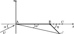
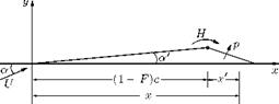
The characteristic of a flapped aerofoil, which is of great importance in stability and control of the aircraft, is the aerodynamic moment about the hinge line, H, shown in Figure 6.10.

Taking moments of elementary pressures p acting on the flap, about the hinge:

trailing edge

H = —
pX dx,

hinge

where:

p = pUk

and:

X = x — (1 — F) c.

Now putting:

X = — (1 — cos 0) — — (1 — cos ф = — ( cos Ф — cos 0)

and k from Equation (6.42), we get the hinge moment as:

H = ~f. 2pU![(“ + ‘0 — C>) ^

Substituting:

H = Ch 2 pU 2(Fc)2

and simplifying, we obtain:

The parameter a1 = dCL/da is 2n and a2 = dCL/dn from Equation (6.43) becomes:

a2 = 2 (n — ф + sin ф). (6.48)

Thus thin aerofoil theory provides an estimate of all the parameters of flapped aerofoil.

The flap at the trailing edge of an aerofoil is essentially a high-lifting device, which when deflected down causes increase of lift, essentially by increasing the camber of the profile. The thin aerofoil discussed in the previous sections of this chapter can readily be applied to aerofoils with variable camber such as flapped aerofoils. It has been found that the circulation distribution along the camber line for the general aerofoil can comfortably be split into the circulation due to a flat plate at an incidence and the circulation due to the camber line.

It is sufficient for the assumptions in the theory to consider the influence of a flap deflection as an addition to the above two components. Figure 6.8 illustrates how the three contributions to lift generation can be combined to get the resultant effect.

‘ n

U

(a)

Indeed the deflection of the flap about a hinge in the camber line effectively alters the camber of the profile so that the contribution due to flap deflection is an addition to the effect of the camber line shape. In this manner, the problem of a cambered aerofoil with flap is reduced to the general case of fitting a camber line made up of the chord of the aerofoil and the flap deflected through an angle n, as shown in Figure 6.9.

The thin aerofoil theory stipulates that the slope of the aerofoil surface is small and that the displacement from the x-axis is small. In other words, the leading and/or trailing edges need not be on the x-axis.

Let us define the camber as hc so that the slope of the part AB of the aerofoil is zero, and the slope of the flap h/F. To find the coefficient of the circulation к for the flap camber, let us substitute these values of slope in Equations (6.32) and (6.34) but confining the limits of integration to the parts of the aerofoil over which the slopes occur. Thus:

ф

where ф is the value of Є at the hinge, that is:

(1 — F) c = 2 (1 — cos ф) ,

hence cos ф = 2F — 1. Integrating Equation (6.39), we get:

ф

A0 = a + n——- (n),

that is:

Similarly, from Equation (6.34):

This gives:

Thus:

2 sin ф sin 2ф

A1 — ——— n and A 2 —————- n.

The chordwise circulation distribution due to flap deflection becomes:

2л Aq + л Aj

giving:

Cl — 2л a + 2(л — ф + sin ф) n.

Likewise, the pitching moment coefficient CMle from Equation (6.36) is:

that is:

In Equations (6.43) and (6.44) ф is given by:

•(1 — F) — ^ (1 — cos ф).

Note that a positive (that is, downward) deflection of the flap decreases the moment coefficient, tending to pitch the aerofoil nose down and vice versa.

From Equation (6.30), the circulation distribution is:

Therefore, the lift becomes:

c

L = pU

П

pU—k sin в de P 2

since:

П

sin в sin пв de = 0 when n = 1.

0

The lift is also given by:

1 2

L = – pU2cCL.

Therefore, the lift coefficient becomes:

The pitching moment is given by:

c

—Mle = pU kxdx

0

1 2 •

= —CMuT. pU c

( 2pU-(c/2)-

Ml‘ ^ 1 pU 2c2

An sin пЄ cos в sin в dв

П П П

= — A0 + — Al — — A2, 2 0 + 2 1 4 2’

Therefore:

A2 Ao + Ai – A
	(6.36)

that is:

The center of pressure coefficient is:

(6.37)

From Equation (6.37) it is seen that for this case also the center of pressure moves as the lift or incidence is changed. We know that the kcp is also given by [Equation (6.19)]:

Comparing Equations (6.36) and (6.37), we get:

This shows that, theoretically, the pitching moment about the quarter chord point for a thin aerofoil is a constant, depending on the camber parameters only, and the quarter chord point is therefore the aerodynamic center.

Example 6.4

The camberline of a thin aerofoil is given by:

y — kx(x – 1)(x – 2),

where x and y are in terms of unit chord and the origin is at the leading edge. If the maximum camber is 2.2% of chord, determine the lift coefficient and the pitching moment coefficient when the angle of attack is 4°.

Solution

Given, camber is 0.022 and a = 4°.

At the maximum camber location, let x = xm. At the maximum camber:

^ = 0,

dx

that is:

k (3xi – 6xm + 2) = 0 3xi – 6x„ + 2 = 0

6 ± V36 – 24
6

1 ± 0.577.

Out of the above two values of 1.577 and 0.423, the second one is the only feasible solution for xm. Therefore, the maximum camber is at xm = 0.423. Substituting this we have:

k[xm(xm – 1)(xm – 2)] = 0.022

k[0.423 x (-0.577) x (-1.577)] = 0.022

But:

(1 – cos в) = 2

Substituting this, we get:

— = – ІЗ cos2 в + 6 cos в – 1І. dx 4 L J

By Equation (6.32):

1

A0 = a——

n

в – 1] de

= a –

33

— k—- k

2 8

Note: The moment is given with a negative sign because this is a nose-down moment.

Example 6.5

A sail plane of wing span 18 m, aspect ratio 16 and taper ratio 0.3 is in level fight at an altitude where the relative density is 0.7. The true air speed measured by an error free air speed indicator is 116 km/h. The lift and drag acting on the wing are 3920 N and 160 N, respectively. The pitching moment coefficient about the quarter chord point is —0.03. Calculate the mean chord and the lift and drag coefficients, based on the wing area and mean chord. Also, calculate the pitching moment about the leading edge of the wing.

Solution

Given 2b = 18 m, = 16, Xt/Xr = 0.3, a = 0.7, L = 3920 N, D = 160 N, Vr = 116 km/h, CMc/4 = -0.03.

The relative density is:

P m a = — = 0.7,

P0

where p0 is the sea level density, equal to 1.225 kg/m3. Therefore:

p = 0.7 P0 = 0.7 x 1.225 = 0.858 kg/m3.

Equivalent air speed is:

V07

= 138.65 km/h _ 138.65 = 3.6

= 38.51 m/s.

The mean chord is:

span

2b

M
18

16

The wing area is:

S = 2b x c = 20.25 m2.

The lift coefficient is:

L

2 pV 2S

2 x 3920

0.858 x 38.512 x 20.25 0.304 .

By Equation (6.36):

The pitching moment about the leading edge is:

1 2

2 pV2 ScCMu

1 x 0.858 x 38.512 x 20.25 x 1.125 x (—0.046) —666.71 Nm.

The negative sign to the moment implies that it is a nose-down moment.

In Section 6.4, we saw that the general camber line can be replaced by a chordwise distribution of circulation. That is:

к — ka + kb,

where ka is the same as the distribution over the flat plate but must contain a constant (A0) to absorb any difference between the equivalent flat plate and the actual chord line. Therefore:

/1 + cos в

ka — 2UAJ ——- . (6.28)

Y sin в J

Note that this ka distribution satisfies the Kutta-Joukowski distribution, since ka — 0 when в — n, that is, at x — c.

The corresponding kb is represented by a Fourier series. Providing 0 < в < n, the end conditions are satisfied, and any variation in shape is accommodated if it is a sine series. Thus:

kb — 2U (Aj sin в + A2 sin 2в + A3 sin 3в + •• ••)

TO

— 2U ‘y ^ An sin пв. (6.29)

Thus, k — ka + kb becomes:

Note that, for circular arc aerofoil, we have kb — 2UA sin в.

The coefficients A0, A1, A2, • • An can be obtained by substituting for k in the general equation

(6.30), suitably converted with regard to units, that is:

Substituting:

c

x = — (1 — cos в),

we get:

Using Equation (6.30), we get:

2U Ґ I A0(1 + cos в) I sin ede

— < ^ ——- – + > An sin пв V———————– .

2n J0 I sin в Г cos в — cos в1

At the point x1 (or в1) on the aerofoil:

dy A0 Гn (1 + cos в) d9 1 Гn An sin пв sin в dв

dx n J0 cos в — cos в; n J0 cos в — cos в;

Expressing У] An sin пв sin в as:

‘У ‘ An — [cos (n — 1) в — cos (n + 1) в] ,

we have:

where Gn signifies the integral:

cos nвdв
cos в — cos в1

which has the solution:

n sin nв1
sin в1

Therefore:

dy A0 sin (n — 1) в; — sin (n + 1) в;

—— a =——— n — > An—————————————

dx n -< 2 sin в;

2 (■

cos в) on the aerofoil, we get:

For the general point x

that is:

On integrating from в = 0 to n, the third term on the right-hand-side of Equation (6.31) vanishes. Therefore, we have:

This simplifies to:

Multiplying Equation (6.32) by cos тв, where m is an integer, and integrating with respect to в, we get:

dy Ґ,

— cos тв de = (a

dx

The integral: ‘y ^ An cos ив cos тв dв = 0.

for all values of n except at n = m. Therefore, the first term on the right-hand-side of Equation (6.33) vanishes, and also the second term, except for n = m becomes:

An cos пЄ
n = —A„
Thus:
(6.34)
An	— cos пЄ dв dx

We know that the lift L, pitching moment about the leading edge of the aerofoil Mle and the pressure p acting on the aerofoil can be expressed as:

1 2

L = – pU 2cCL

Mie = 2 pU 2c2Cmic p = pUk.

Now, substituting:

the pressure becomes:

Also,

x = — (1 — cos в).

Therefore, the lift becomes:

L = I pdx

П _

= — pU2c 2 І а(1 + cos в) + 2вsin2 в

that is:

The lift coefficient is:

L

2 pU 2c

This gives:

Thus the lift-curve slope is:

From the above relations for CL and dCL /da, it is evident that:

at a = 0, CL = 2пв at a = —в, CL = 0

and the lift-curve slope is independent of camber.

For a cambered aerofoil, we have:

2л (a + в)

dCL

ЮГ(a

For CL = 0, a = —в or —aL=0 = в. Thus:

The pitching moment is:

Mie = — pxdx

0

= —2pU2c2f (a + 2в).

Therefore, the pitching moment coefficient becomes:

In terms of CL, the CMle can be expressed as follows. By Equation (6.23a), we have the CL as:

Cl = 2n (a + в).

The expression for CMle, in Equation (6.25), can be arranged as:

But CL = 2п (a + в), thus:

1

Cm“ = —2

or

The center of pressure coefficient, kcp, becomes:

Thus, the effect of camber is to set back the center of pressure by an amount which decreases with increasing incidence or lift. At zero lift, the center of pressure is an infinite distance behind the aerofoil, which means that there is a moment on the aerofoil even when there is no resultant lift force.

Comparing this with Equation (6.17a) (CMle =— |a) for flat plate we see that the camber of circular arc decreases the moment about the leading edge by пв/2.

Example 6.3

(a) A flat plate is at an incidence of 2° in a flow; determine the center of pressure. (b) If a circular arc of 3% camber is in the flow at the same incidence, where will be center of pressure?

Solution

(a) Given, a = 2°.

For a flat plate, by Equation (6.16), the lift coefficient is:

CL = 2пa

= 2п x (2 x —— 2

V 180/

= 0.219.

By Equation (6.17):

Aliter:

Note that the kcp is also given by Equation (6.27), as:

1 n в = 4 + 2CL 1 i n x 0.06 — 4 + 2 x 0.596 = 0.408.

This is the same as that given by dividing CMle with CL.