Category THEORETICAL AERODYNAMICS

Following the same procedure as before for finding the distribution of k, it can be shown that for a circular arc aerofoil at an angle of attack a to the flow k can be expressed as:

From Equations (6.12) and (6.14) is seen that the effect of camber is to increase k distribution by (2U x 2в sin в) over that of the flat plate. Thus:

k — ka + kbі

arises from the incidence of the aerofoil alone and:

which is due to the effect of the camber alone. Note that this distribution satisfies the Kutta-Joukowski hypothesis by allowing k to vanish at the trailing edge of the aerofoil where в = n.

Example 6.2

If the maximum circulation caused by the camber effect of a circular arc aerofoil is 2 m2/s, when the freestream velocity is 500 km/h, determine the percentage camber.

Solution

Given, kb = 2 m2/s, U = 500/3.6 = 138.9 m/s.

By Equation (6.22), the circulation due to camber is:

kb = 4ив sin в.

This circulation will be maximum when sin в = 1, thus:

kbmax = 4UP.

Therefore:

kbmax

4U

_ 2 = 4 x 138.9 = 0.0036.

The % camber becomes:

%Camber = — x 100

0.0036

2

The expression for k can be put in the equations for lift and pitching moment, by using the pressure:

(1 cos в)

p = pUk = 2pU2a—————– . (6.15)

sin в

It is to be noted that:

• Full circulation is involved in k.

• The circulation k vanishes at the trailing edge, where x = c and в = n. This must necessarily be so for the velocity at the trailing edge to be finite.

The lift per unit span is given by:

For small values of angle of attack, a, the center of pressure coefficient, kcp, (defined as the ratio of the center of pressure from the leading edge of the chord to the length is chord), is given by:

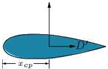
This shows that the center of pressure, which is a fixed point, coincides with the aerodynamic center. This is true for any symmetrical aerofoil section. The resultant force at the leading edge, at the quarter chord point and the center of pressure of a symmetrical aerofoil are shown in Figure 6.6.

By inspection, the quantitative relation between the three cases shown in Figure 6.6 can be expressed as:

Figure 6.6 Resultant force on a symmetrical aerofoil.

Thus, the momentum coefficient about the quarter-chord point is:

This is the theoretical result that “the center of pressure is at the quarter-chord point for a symmetrical aerofoil.”

By definition the point on the aerofoil where the moments are independent of angle of attack is called the aerodynamic center. The point from the leading edge of the aerofoil at which the resultant pressure acts is called the center of pressure. In other words, center of pressure is the point where line of action of the lift L meets the chord. Thus the position of the center of pressure depends on the particular choice of chord.

The center of pressure coefficient is defined as the ratio of the center of pressure from the leading edge of the aerofoil to the length of chord. This is represented by the symbol kcp. One of the desirable properties of an aerofoil is that the travel of center of pressure in the working range of incidence (that is from zero-lift incidence to the stalling incidence) should not be large. As incidence increases the center of pressure moves towards the quarter-chord point.

From the above result, it is seen that the moment about the quarter-chord point is zero for all values of a. Hence, for a symmetrical aerofoil, we have the theoretical result that “the quarter-chord point is both the center of pressure and the aerodynamic center.” In other words, for a symmetrical aerofoil the center of pressure and aerodynamic center overlap. That is, for a symmetrical aerofoil the center of pressure and aerodynamic center coincide.

The relative position of center of pressure cp and aerodynamic center ac plays a vital role in the stability and control of aircraft. Let us have a closer look at the positions of cp and ac, shown in Figure 6.7.

We know that the aerodynamic center is located around the quarter chord point, whereas the center of pressure is a moving point, strongly influenced by the angle of attack. When the center of pressure is aft of aerodynamic center, as shown in Figure 6.7(a), the aircraft will experience a nose-down pitching moment. When the center of pressure is ahead of aerodynamic center, as shown in Figure 6.7(b), the aircraft will experience a nose-up pitching moment. When the center of pressure coincided with the aerodynamic center, as shown in Figure 6.7(c), the aircraft becomes neutrally stable.

From our discussions on center of pressure and aerodynamic center, the following can be inferred:

• “Center of pressure” is the point at which the pressure distribution can be considered to act-analogous to the “center of gravity” as the point at which the force of gravity can be considered to act.

• The concept of the “aerodynamic center” on the other hand, is not very intuitive. Because the lift and location of the center of pressure on an airfoil both vary linearly (more or less) with angle of attack, a, at least within the unstalled range of a. That is we can define a point on the chord of the airfoil at which the pitching moment remains “constant,” regardless of the a. That point is usually near the quarter-chord point and for a symmetrical airfoil the constant pitching moment would be zero. For a cambered airfoil the pitching moment about the aerodynamic center would be nonzero, but constant. The usefulness of the aerodynamic center is in stability and control analysis where the aircraft can be defined in terms of the wing and tail aerodynamic centers and the required lift and moments calculated without worrying about the shift in center of pressure with a.

The horizontal position of the center of gravity has a great effect on the static stability of the wing, and hence, the static stability of the entire aircraft. If the center of gravity is sufficiently forward of the aerodynamic center, then the aircraft is statically stable. If the center of gravity of the aircraft is moved toward the tail sufficiently, there is a point – the neutral point – where the moment curve becomes horizontal; this aircraft is neutrally stable. If the center of gravity is moved farther back, the moment curve has positive slope, and the aircraft is longitudinally unstable. Likewise, if the center of gravity is moved forward toward the nose too far, the pilot will not be able to generate enough force on the tail to raise the angle of attack to achieve the maximum lift coefficient.

The horizontal tail is the main controllable moment contributor to the complete aircraft moment curve. A larger horizontal tail will give a more statically stable aircraft than a smaller tail (assuming, as is the normal case, that the horizontal tail lies behind the center of gravity of the aircraft). Of course, its distance from the center of gravity is important. The farther away from the center of gravity it is, the more it enhances the static stability of the aircraft. The tail efficiency factor depends on the tail location with respect to the aircraft wake and slipstream of the engine, and power effects. By design it is made as close to 100% efficiency as possible for most static stability.

Finally, with respect to the tail, the downwash from the wing is of considerable importance. Air is deflected downward when it leaves a wing, and this deflection of air results in the wing reaction force or lift. This deflected air flows rearward and hits the horizontal-tail plane. If the aircraft is disturbed, it will change its angle of attack and hence the downwash angle. The degree to which it changes directly affects the tail’s effectiveness. Hence, it will reduce the stability of the airplane. For this reason, the horizontal tail is often located in a location such that it is exposed to as little downwash as possible, such as high on the tail assembly.

The problem now is to express the vorticity distribution k as some expression in terms of the camber line shape. Another method of finding kdx is to utilize the method of Equation (6.9), where simple expressions can be found for the velocity distribution around skeleton aerofoils. The present approach is to work up to the general case through particular skeleton shapes that do provide such simple expressions, and then apply the general case to some practical considerations.

6.1.1 Thin Symmetrical Flat Plate Aerofoil

For a flat plate, dy/dx = 0. Therefore, the general equation [Equation (6.9)] simplifies to:

1 fc kdx

Ua = — ———- .

2n J0 —x + X1

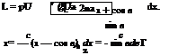
It is convenient to express the variable x in terms of в, through:

c

x = — (1 — cos в)

and x1 in terms of в1 as:

c

x1 = ^(1 — cos в1).

The integration limits of Equation (6.10) become:

в varies from 0 to n (that is, 0 < в < n) as x varies from 0 to c (that is, 0 < x < c)

and

dx = – sin в de. 2

Equation (6.10) becomes:

A value of k which satisfies Equation (6.11) is:

(1 + cos в)
sin в

Therefore:

A more direct method for getting the vorticity distribution k is found as follows.

Transformation of the circle z = aelB, through the Joukowski transformation Z = z + , to a lifting

flat plate section at an incident angle a requires by the Joukowski hypothesis that sufficient circulation be

imposed to bring the rear stagnation point down to m on the cylinder, as shown in Figure 6.5(a), where the velocity at a given point P(a, в) is:

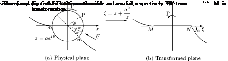
qa =

that is:

For small a this simplifies to:

The variable в in Equation (6.13) is the same as that used in the general equation [Equation (6.11)]. This can be easily shown by shifting the axes in Figure 6.5(b) to the leading edge and measuring x rearward. When the chord c = 4a, the distance x becomes:

c

= 2

c

= 2 (1 – cos в) .

Then taking:

k — qa1 qa2 .

where qa1 is the velocity at the point where в = в1 and qa2 is the velocity at the same point on the other side of the aerofoil where в = —в. Therefore:

Thus, in general, the elementary circulation at any point on the flat plate is:

Example 6.1

(a) Find the circulation at the mid-point of a flat plate at 2° to a freestream of speed 30 m/s.

(b) Will this be greater than or less than the circulation at the quarter chord point?

Solution

(a) Given, a = 2°, U = 30 m/s.

At the mid-point of the plate в = n/2.

Circulation around a plate at a small angle of incidence, by Equation (6.14), is:

At в = n/2, the circulation is:

k = 2 x 30 x (2 x 180)

(b) The coordinate along the plate is:

§ = 2b cos в.

At the quarter chord point, § = 3b/4, since chord is 4b and the chord is measured from в = n, that is, from the trailing edge. Thus:

3b/4 = 2b cos в 3

в = cos
= 68°.

Therefore, the circulation at the quarter chord point becomes:

, n /1 + cos 68°

k = 2 x 30 x 2 x ——— ) x ——————

18^ V sin 68°

= 3.105 m2/s.

The circulation at the quarter chord point is greater than that at the middle of the plate.

This theory is based on the assumption that the aerofoil is thin so that its shape is effectively that of its camber line and the camber line shape deviates only slightly from the chord line. In other words, the

Figure 6.3

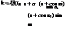
theory should be restricted to low angles of incidence. The modification to the aerofoil theory with the above simplifications are the following:

• Replacement of the camber line by a string of line vortices of infinitesimal strengths, as shown in Figure 6.3(a).

• The camber line is replaced by a line of variable vorticity so that the total circulation about the chord is the sum of the vortex elements. Thus, the circulation around the camber becomes:

Г = f kSs, (6.1)

J0

where k is the vorticity distribution over the element of camber line, Ss, circulation is taken positive (+ve) in the clockwise direction, as shown in Figure 6.3(a), and c is the chord of the profile.

Following Glauert, the leading edge is taken as the origin, ox along the chord and oy normal to it. The basic assumptions of the theory permit the variation of vorticity along the camber line be assumed to be the same as the variation along ox-axis, that is, Ss differs negligibly from Sx. Therefore, the circulation can be expressed as:

Г = I kdx. (6.2)

0

Hence the lift per unit span is given by:

L = pUr = pU I kdx. (6.3)

0

With pUk = p, Equation (6.3) can be written as:

•c

Again for unit span, p has the units of force per unit area or pressure and the moment of these chordwise pressure forces about the leading edge or origin of the system is:

c

The negative sign for Me in Equation (6.5) is because it is conventional to take the nose-down moment as negative and nose-up moment as positive. For an aircraft in normal flight with lift acting in the upward direction, the moment about the leading edge of the wing will be nose-down. Thus, the thin wing section has been replaced by a line discontinuity in the flow in the form of a vorticity distribution. This gives rise to an overall circulation, as does the aerofoil, and produces a chordwise pressure variation. The static pressures p1 and p2 above and below the element Ss at a location with velocities (U + u{), (U + u2), respectively, over the upper and lower surfaces, are as shown in Figure 6.3(b). The overall pressure difference is (p2 — p1). By incompressible Bernoulli equation, we have:

1 , ,2 1 2

p1 + 2 P (U + U1) = p<x> + 2 pu

1 , ,2 1 2

p2 + 2P (U + u2) = p<x> + 2pU ’

where px is the freestream pressure. Therefore the overall pressure difference becomes:

For a thin aerofoil at small incidence, the perturbation velocity ratios u1/U and u2/U will be very small, and therefore, higher order terms can be neglected. Therefore, the overall pressure difference simplifies to:

The equivalent vorticity distribution indicates that the circulation due to the element Ss is kSx (Ss is replaced with Sx because the camber line deviates only slightly from the ox-axis).

Evaluating the circulation around Ss and taking clockwise circulation as positive in this case and by taking the algebraic sum of the flow of fluid along the top and bottom of Ss, we get:

kSx = (U + U1)Sx — (U + u2)Sx = (u1 — U2)S.

From Equations (6.6) and (6.7), it is seen that p = pUk, as introduced earlier.

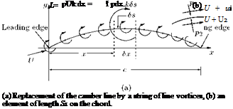
The flow direction everywhere on the aerofoil must be tangential to the surface and makes an angle tan-1 (dy/dx), since the aerofoil is thin, the angle dy/dx from ox-axis is as shown in Figure 6.4.

Resolving the vertical velocity components, we have:

since both dy/dx and a are small, tan dx approximated as ddx and sin a is approximated as a. Ignoring the second-order quantities, we can express the above equation as:

(6.8)

The induced velocity v is found by considering the effect of the elementary circulation kSx at x, a distance (x — xj) from the point considered.

Circulation kSx induces a velocity at the point x1 equal to:

The effect of all such elements of circulation along the chord is the induced velocity v, where:

Using Equation (6.8) this becomes:

(6.9)

The solution of kdx which satisfies Equation (6.9) for a given shape of camber line (defining dy/dx) and incidence can be introduced in Equation (6.4) and (6.5) to obtain the lift L and pitching moment M for the aerofoil shape. That is, using this circulation distribution (kdx), the lift and pitching moment can be calculated with Equations (6.4) and (6.5), respectively. From these L and Me, the lift coefficient CL and pitching moment coefficient CMu can be determined. Thus, once the circulation distribution is known, the characteristic lift coefficient CL and pitching moment coefficient CMu follow directly and hence the center of pressure coefficient, kcp and the angle of zero lift.

6.1 Introduction

The main limitation of Joukowski’s theory is that it is applicable only to the Joukowski family of aerofoil sections. Similar is the case with aerofoils obtained with other transformations. These aerofoils do not permit a satisfactory solution of the reverse problem of aerofoil design, that is, to start with the loading distribution and from the loading, obtain the necessary aerofoil profile. For the indirect or reverse solution to be possible, a theory which consists of more local relationships is required. That is:

• The overall lifting property of a two-dimensional aerofoil depends on the circulation it generates and this, for the far-field or overall effects, has been assumed to be concentrated at a point within the aerofoil profile, and to have a magnitude related to the incidence, camber and thickness of the aerofoil.

• The loading on the aerofoil, or the chordwise pressure distribution, follows as a consequence of the parameters, namely the incidence, camber and thickness. But the camber and thickness imply a characteristic shape which depends in turn on the conformal transformation function and the basic flow to which it is applied.

• The profiles obtained with Joukowski transformation do not lend themselves to modern aerofoil design.

• However, Joukowski transformation is of direct use in aerofoil design. It introduces some features which are the basis to any aerofoil theory, such as:

(a) The lift generated by an aerofoil is proportional to the circulation around the aerofoil profile, that is, L а Г.

(b) The magnitude of the circulation Г must be such that it keeps the velocity finite in the vicinity of trailing edge.

• It is not necessary to concentrate the circulation in a single vortex, as shown in Figure 6.1(a), and an immediate extension to the theory is to distribute the vorticity throughout the region surrounded by the aerofoil profile in such a way that the sum of the distributed vorticity equals that of the original model, as shown in Figure 6.1(b), and the vorticity at the trailing edge is zero.

This mathematical model may be simplified by distributing the vortices on the camber line and disre­garding the effect of thickness. In this form it becomes the basis for the classical “thin aerofoil theory” of Munk and Glauert.

2

Considering the fact that the transformation Z = г + Z applied to a circle in an uniform stream gives a straight line aerofoil (that is, a flat plate), the theory assumed that the general thin aerofoil could be

Theoretical Aerodynamics, First Edition. Ethirajan Rathakrishnan.

© 2013 John Wiley & Sons Singapore Pte. Ltd. Published 2013 by John Wiley & Sons Singapore Pte. Ltd.

a camber line.

replaced by its camber line, which is assumed to be only a slight distortion of a straight line. Consequently the shape from which the camber line has to be transformed would be a similar distortion from the original circle. The original circle could be found by transforming the slightly distorted shape, shown in Figure 6.2.

This transformation function defines the distortion, or change of shape, of the circle, and hence by implication, the distortion (or camber) of the straight line aerofoil. As shown in Figure 6.2, the circle (z = ae’e) inthez-plane is transformed to the “S” shape in the z’-plane using the transformation z! = f (z), and then the S shape to a cambered profile using the following transformation:

Z = z’ + –

z

и

= f (z) + 7Й’

It is evident that z’ = f (z) defines the shape of the camber and Glauert used the series expansion:

z’ = z 1 +

for this. Using potential theory and Joukowski hypothesis, the lift and pitching moment acting on the aerofoil section were found in terms of the coefficients Ax, that is in terms of the shape parameter.

The usefulness or advantage of the theory lies in the fact that the aerofoil characteristics could be quoted in terms of the coefficient Ax , which in turn could be found by graphical integration method from any camber line.

1. Evaluate the vorticity of the following two-dimensional flow.

(i) u = 2xy, v = x2.

(ii) u = x2, v = —2xy.

(iii) ur = 0, Ug = r.

(iv) Ur = 0, Ug = 1.

[Answer: (i) 0, (ii) —2(x + y), (iii) 2, (iv) 0]

2. If the velocity induced by a rectilinear vortex filament of length 2 m, at a point equidistant from the extremities of the filament and 0.4 m above the filament is 2 m/s, determine the circulation around the vortex filament.

[Answer: 5.414 m2/s]

3. A point P in the plane of a horseshoe vortex is between the arms and equidistant from all the filaments. Prove that the induced velocity at P is:

Г(1 + V2)

v =————– ,

nAB

where Г is the intensity and AB is the length of the finite side of the horseshoe.

Ш Figure 5.59 A sprinkler.

4. If the velocity induced by an infinite line vortex of intensity 100 m2/s, at a point above the vortex is 40 m/s, determine the height of the point above the vortex line.

[Answer: 0.398 m]

5. If a wing of span 18 m has a constant circulation of 150 m2/s around it while flying at 400 km/h, at sea level, determine the lift generated by the wing.

[Answer: 367.5 kN]

6. If the tangential velocity at a point at radial distance of 1.5 m from the center of a circular vortex is 35 m/s, determine (a) the intensity of the vortex and (b) the potential function of the vortex flow.

[Answer: (a) 329.87 m2/s, (b) 52.5 9]

7. Show that a circular vortex ring of intensity Г induces an axial velocity 2R at the center of the ring, where R is the radius of the vortex.

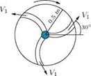
8. A rotating device to sprinkle water is shown in Figure 5.59. Water enters the rotating device at the center at a rate of 0.03 m3/s and then it is directed radially through three identical channels of exit area 0.005 m2 each, perpendicular to the direction of flow relative to the device. The water leaves at an angle of 30° relative to the device as measured from the radial direction, as shown. If the device rotates clock wise with a speed of 20 radians/s relative to the ground. Compute the magnitude of the average velocity of the fluid leaving the vane as seen from the ground.

[Answer: 9.16 m/s, at an angle of 79° with respect to the ground (horizontal)]

9. Determine an expression for the vorticity of the flow field described by:

V = x2yi — xy2 j.

Is the flow irrotational?

[Answer: Z = Zzk = — (x2 + y2) k. The flow is not irrotational, since the vorticity is not zero.]

10. When a circulation of strength Г is imposed on a circular cylinder placed in an uniform incompressible flow of velocity Ux, the cylinder experiences lift. If the lift coefficient CL = 2, calculate the peak (negative) pressure coefficient on the cylinder.

[Answer: — 4.373]

11. A wing with an elliptical planform and an elliptical lift distribution has aspect ratio 6 and span of 12 m. The wing loading is 900 N/m2, when flying at a speed of 150 km/hr at sea level. Calculate the induced drag for this wing.

[Answer: 969.44 N]

12. A free vortex flow field is given by v = , for r > 0. If the flow density p = 103 kg/m3 and the

2nr

volume flow rate q = 20n m2/s, express the radial pressure gradient, dp/dr, as a function of radial distance r, and determine the pressure change between ri = 1m and r2 = 2 m.

Answer: —r^, 37.5 kPa

r3

13. A viscous incompressible fluid is in a two-dimensional motion in circles about the origin with tangential velocity:

1 (r2

Щ = – f — r vt

where v is kinematic velocity and t is time. Find the vorticity f.

14.

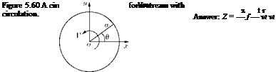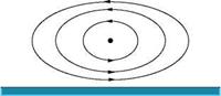
A circular cylinder of radius a is in an otherwise uniform stream of inviscid fluid but with a positive circulation round the cylinder, as shown in Figure 5.60. Find the lift and drag per unit span of the cylinder. Also, sketch the streamlines around the cylinder if the circulation is subcritical.

[Answer: lift = рУ^Г, drag = 0]

15. A square ring vortex of side 2a. If each side has strength Г, calculate the velocity induced at the center of the ring.

V2

Answer: — Г

References

1. Rathakrishnan, E., Fluid Mechanics – An Introduction, 3rd edn. PHI Learning, New Delhi, 2012.

2. Milne-Thomson, L. M., Theoretical Aerodynamics, 2nd edn. Macmillan & Co., Ltd, London, 1952.

3. Lamb, H., Hydrodynamics, 6th edn. Dover Publications, 1932.

4. Rathakrishnan, E., Applied Gas Dynamics, John Wiley, NJ, 2010.

Consider a continuous distribution of vortices on a straight line AB stretching from (—c/2, 0) to (c/2, 0), as shown in Figure 5.58.

Let the elements d§ of the line at point (§, 0) behave like a point rectilinear vortex of strength yd%, where у may be constant or a function of §. This element taken by itself will induce at the point P(x, 0) a velocity of dvx, in the negative y-direction, as shown in Figure 5.58, given by:

Yd§

§ – x

Thus the whole line of vortices will induce at P the velocity:

Note that in Equation (5.79), § is a variable and x is fixed. When § = x, the integrand is infinite. On the other hand, using the principle that a vortex induces no velocity at its own center, the point x must be omitted from the range of variation of §. To do this we define the “improper” integral Equation (5.79) by its “principal value,” namely:

In this way the point (x, 0) is always the center of the omitted portion between (x — є) and (x + e).

In the theory of aerofoil the type of integral (Equation 5.80) in which we shall be interested is that for which § =—Ic cos ф and y = Yn sin пф where Yn is independent of ф.

Now let x =—1 c cos в, where в, like x, is fixed. We get from Equation (5.79):

sin пф sin фdф

0 cos в — cos ф

1 Ґ [cos (n — 1) ф — cos (n + 1) ф] dф

2^n J0 cos в — cos ф

In this relation, we have integral of the type:

cos пф

—Ъ——— т Лф.

cos в — cos ф

5.20 Summary

The following are the three possible ways in which a fluid element can move.

(a) Pure translation – the fluid elements are free to move anywhere in space but continue to keep their axes parallel to the reference axes fixed in space.

(b) Pure rotation – the fluid elements rotate about their own axes which remain fixed in space.

(c) The general motion in which translation and rotation are compounded.

A flow in which all the fluid elements behave as in item (a) above is called potential or irrotational flow. All other flows exhibit, to a greater or lesser extent, the spinning property of some of the constituent fluid elements, and are said to posses vorticity, which is the aerodynamic term for elemental spin. The flow is then termed rotational Bow.

The angular velocity is given by:

dv du 2o) = .

dx dy

The quantity 2o) is the elemental spin, also referred to as vorticity, Z. Thus:

The units of Z are radian per second. It is seen that:

that is, the vorticity is twice the angular velocity.

In the polar coordinates, the vorticity equation can be expressed as:

where r and в are the polar coordinates and qt and qn are the tangential and normal components of velocity, respectively.

Circulation is the line integral of a vector field around a closed plane curve in a flow field. By definition:

Circulation implies a component of rotation of flow in the system. This is not to say that there are circular streamlines, or the elements, of the fluid are actually moving around some closed loop although this is a possible flow system. Circulation in a flow means that the flow system could be resolved into an uniform irrotational portion and a circulating portion.

If circulation is present in a fluid motion, then vorticity must be present, even though it may be confined to a restricted space, as in the case of the circular cylinder with circulation, where the vorticity at the center of the cylinder may actually be excluded from the region of flow considered, namely that outside the cylinder.

The sum of the circulations of all the elemental areas in the circuit constitutes the circulation of the circuit as a whole:

Vorticity = lim ———————- .

area^0 area of element

A line vortex is a string of rotating particles. In a line vortex, a chain of fluid particles are spinning about their common axis and carrying around with them a swirl of fluid particles which flow around in circles.

Vortices can commonly be encountered in nature. The difference between a real (actual) vortex and theoretical vortex is that the real vortex has a core of fluid which rotates like a solid, although the associated swirl outside is the same as the flow outside the point vortex. The streamlines associated with a line vortex are circular, and therefore, the particle velocity at any point must be only tangential.

The stream function for a vortex is:

The potential function ф for a vortex is:

A vortex is a Bow system in which a finite area in a plane normal to the axis of a vortex contains vorticity. The axis of a vortex, in general, is a curve in space, and area S is a finite size. It is convenient to consider that the area S is made up of several elemental areas. In other words, a vortex consists of a bundle of elemental vortex lines or filaments. Such a bundle is termed a vortex tube, being a tube bounded by vortex filaments.

The four fundamental theorems governing vortex motion in an inviscid flow are called Helmholtz’s theorems.

Helmholtz’s first theorem states that:

“the circulation of a vortex tube is constant at all cross-sections along the tube."

The second theorem demonstrates that:

“the strength of a vortex tube (that is, the circulation) is constant along its length."

This is sometimes referred to as the equation of vortex continuity. It follows from the second theorem that Z S is constant along the vortex tube (or filament), so that if the cross-sectional area diminishes, the vorticity increases and vice versa. Since infinite vorticity is unacceptable, the cross-sectional area S cannot diminish to zero. In other words, a vortex cannot end in the fluid. In reality the vortex must form a closed loop, or originate (or terminate) in a discontinuity in the fluid such as a solid body or a surface of separation. In a different form it may be stated that a vortex tube cannot change its strength between two sections unless vortex filaments of equivalent strength join or leave the vortex tube.

The third theorem demonstrates that a vortex tube consists of the same particles of fluid, that is:

“there is no fluid interchange between the vortex tube and surrounding fluid."

The fourth theorem states that:

“the strength of a vortex remains constant in time."

By definition (Equation 5.3), we have the circulation as:

Г = ф V ■ ds.

The time rate of change of Г can be expressed as:

By Euler equation, we have:

Thompson’s vortex theorem or Kelvin’s circulation theorem states that:

“in a flow of inviscid and barotropic fluid, with conservative body forces, the circulation around a closed curve (material line) moving with the fluid remains constant with time, " if the motion is observed from a nonrotating frame.

The vortex theorem can be interpreted as follows:

“The position of a curve c in a flow field, at any instant of time, can be located by following the motion of all the fluid elements on the curve. "

That is, Kelvin s circulation theorem states that the circulation around the curve c at the two locations is the same. In other words:

where D/Dt(= d/dt + V ■) has been used to emphasize that the circulation is calculated around a material contour moving with the fluid.

With Kelvin’s theorem as the starting point, we can explain the famous Helmholtz’s vortex theorem, which allows a vivid interpretation of vortex motions which are of fundamental importance in aerodynamics.

The lift per unit span of an aerofoil can be expressed as:

where p and V, respectively, are the density and velocity of the freestream flow.

A closed line which surrounds only the vortex has a fixed circulation and must necessarily cross the discontinuity surface. Therefore, Kelvin’s circulation theorem does not hold for this line. A curve which surrounds the aerofoil only has the same circulation as the free vortex, but with opposite sign, and therefore the aerofoil experiences a lift. The circulation about the aerofoil with a vortex lying over the aerofoil, due to the boundary layer at the surface, is called the bound vortex.

The Stoke’s integral theorem states that:

“The line integral J u ■ dx about the closed curve c is equal to the surface integral JJ (y x u) ■ nds over any surface of arbitrary shape which has c as its boundary."

That is, the surface integral of a vector field u is equal to the line integral of u along the bounding curve:

where dx is an elemental length on c, and n is unit vector normal to any elemental area on ds. Helmholtz’s first vortex theorem states that:

“the circulation of a vortex tube is constant along the tube. "

A vortex tube is a tube made up of vortex lines which are tangential lines to the vorticity vector field, namely curl u (or f).

In an irrotational vortex (free vortex), the only vortex line in the flow field is the axis of the vortex. In a forced vortex (solid-body rotation), all lines perpendicular to the plane of Bow are vortex lines.

The integral:

(curlu) ■ nds

is called the vortex strength. It is identical to the circulation.

A very thin vortex tube is referred to as a vortex filament. The vortex filaments are of particular importance in aerodynamics. The angular velocity increases with decreasing cross-section of the vortex filament.

is an inhomogeneous Laplace equation, also called Poisson’s equation. The theory of this partial dif­ferential equation is the subject of potential theory which plays an important role in many branches of physics as in fluid mechanics.

Biot-Savart law relates the intensity of magnitude of magnetic field close to an electric current carrying conductor to the magnitude of the current. It is mathematically identical to the concept of relating

intensity of flow in the fluid close to a vorticity-carrying vortex tube to the strength of the vortex tube. It is a pure kinematic law, which was originally discovered through experiments in electrodynamics. The vortex filament corresponds there to a conducting wire, the vortex strength to the current, and the velocity field to the magnetic field. The aerodynamic terminology namely, “induced velocity” stems from the origin of this law.

The induced velocity is given by:

Г

v = —– (1 — cos в) .

4nr

The velocity induced at P by the element of length Ss is:

The induced velocity at a point P above vortex AB is:

where a = ZPAB and в = ZPBA.

A vortex is termed semi-infinite vortex when one of its ends stretches to infinity. The velocity induced by a semi-infinite vortex at a point P:

v =—— (cos a + 1) ,

4nh

where a = ZPAB and end B tends to infinity.

An infinite vortex is that with both ends stretching to infinity. For this case we have a = в = 0. Thus, the induced velocity due to an infinite vortex becomes:

_ Г 2nh

For a specific case of point P just opposite to one of the ends of the vortex, say A, we have a = n/2 and cos a = 0. Thus, the induced velocity at P becomes:

_ Г 4nh

The circulation of the vortex determines the lift, and the lift formula which gives the relation between circulation, Г, and lift per unit width, l, in inviscid potential flow is the Kutta-Joukowski theorem.

The Kutta-Joukowski theorem states that “the force per unit length acting on a right cylinder of any cross section whatsoever is equal to px УОТГОТ, and is perpendicular to the direction of VOT,” namely:

l = — рГи^,

where l is the lift per unit span of the wing, Г is circulation around the wing, is the freestream velocity and p is the density of the flow.

The lift of the whole wing span 2b is given by:

If a long time has passed since start-up, the starting vortex is at infinity (far downstream of the wing), and the bound vortex and the tip vortices together form a horseshoe vortex.

The velocity w induced at the middle of the wing by the two tip vortices accounts to double the velocity induced by a semi-infinite vortex filament at distance b. Therefore:

Г, ч Г

w = —— (1 + 0) = ——- .

4nb 4nb

This velocity is directed downwards and hence termed induced downwash.

The induced drag Di, given by:

w

Di = A—— .

‘ Uoo

The flow outside the vortex filament is a potential flow. Thus, by incompressible Bernoulli equation, we have:

The second vortex theorem of Helmholtz’s states that:

“a vortex tube is always made up of the same fluid particles."

In other words, a vortex tube is essentially a material tube. This characteristic of a vortex tube can be represented as a direct consequence of Kelvin’s circulation theorem.

The third vortex theorem of Helmholtz’s states that:

“the circulation of a vortex tube remains constant in time."

Using Helmholtz’s second theorem and Kelvin’s circulation theorem, the above statement can be inter­preted as “a closed line generating the vortex tube is a material line whose circulation remains constant.” Helmholtz’s second and third theorems hold only for inviscid and barotropic fluids.

The fourth theorem states that:

“the strength of a vortex remains constant in time."

This is similar to the fact that the mass flow rate through a streamtube is invariant as the tube moves in the flow field. In other words, the circulation distribution gets adjusted with the area of the vortex tube. That is, the circulation per unit area (that is, vorticity) increases with decrease in the cross-sectional area of the vortex tube and vice versa.

Vortex is a fluid flow in which the streamlines are concentric circles. The vortex motions encountered in practice may in general be classified as free vortex or potential vortex and forced vortex or flywheel vortex.

Forced vortex is a rotational flow field in which the fluid rotates as a solid body with a constant angular velocity ю, and the streamlines form a set of concentric circles. Because the fluid in a forced vortex rotates like a rigid body, the forced vortex is also called flywheel vortex. The free surface of a forced vortex is in the form of a paraboloid.

Free vortex is an irrotational flow field in which the streamlines are concentric circles, but the variation of velocity with radius is such that there is no change of total energy per unit weight with radius, so that dH/dr = 0. Since the flow field is potential, the free vortex is also called potential vortex.

For a free vortex, the tangential velocity becomes:

This shows that in the flow around a vortex core the velocity is inversely proportional to the radius.

In a free vortex, pressure decreases and circumferential velocity increases as we move towards the center.

A free spiral vortex is essentially the combination of a free cylindrical vortex and a radial flow.

Flow in which the fluid flows radially inwards, or outwards from a center is called a radial flow.

A free spiral vortex is that in which a fluid element will follow a spiral path.

A rectilinear vortex is a vortex tube whose generators are perpendicular to the plane of motion.

A circular vortex is that with the shape of its cross-section normal to its axis of rotation as circular.

The existence of a vortex implies the co-existence of certain distribution of velocity field. This velocity field which co-exists with the vortex is known as the induced velocity field and the velocity at any point of it is called the induced velocity.

A circular vortex induces zero velocity at its center. Thus, a circular vortex alone in the otherwise undisturbed fluid will not tend to move.

Naturally occurring tropical cyclone, hurricane and typhoon which attains a diameter of from 150 to 800 kilometers, and travels at a speed seldom exceeding 25 kilometer per hour are circular vortices on a large scale. Within the area the wind can reach hurricane force, while there is a central region termed “the eye of the storm" of diameter about 15-30 kilometers where conditions may be completely calm.

Point rectilinear vortex is the limiting case of a circular vortex of constant strength у with radius a tending to zero.

Two vortices of equal strength у but opposite nature (one rotating clockwise and the other rotating counterclockwise) from a vortex pair.

Consider two vortices of strength у and y’ located at (0, 0) and (0, h), as shown in Figure 5.56. These two vortices repel one another if у and y’ have the same sign, and attract if the signs are opposite. This result has its application to the action between the vortices shed by the wings of a biplane.

5.19 Energy due to a Pair of Vortices

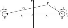
Consider two circular vortices of equal radius a and equal strength у placed as shown in Figure 5.57 with the distance 2b between their centers very large compared to a, so that their circular form is preserved.

l/h

h

Y /h

Figure 5.56 Two vortices at a finite distance between them.

Neglecting the interaction between them, we can write the vorticity as:

Z = iy ln (z — b) — iy ln (z + b)

The stream function is:

ф = у ln (—

Г2

where ri, r2 are the distance of the point z from the vortices, as shown in Figure 5.57. For the region external to the vortices the kinetic energy of the fluid is:

KEo = — p I I (u2 + v2) dxdy.

Now in terms of stream function ф:

2 2 дф дф

u2 + v = u——— v —

dy dx

д(иф) д(vф) du dv

ду дх ду дх

д^ф) дфф) (дv дu

ду дх + ^ 1 дх ду

But the region outside the vortices is irrotational and hence vorticity:

дv дu ^ дх ду

Thus,

Therefore, we have:

1

KE0 = 2 p x 2
(цф dx + уф dy).

The integration is taken positively (in the counterclockwise direction) round c, and the circumference of the vortex at z = b. The factor 2 is to account for the two vortices contributing the same amount to the energy.

Now:

u dx + vdy = Vsds,

where Vs is the speed tangential to contour c and ds is arc length along c. Therefore:

Vs ds = 2ny the circulation.

Also, on c, r1 = a, and r2 = 2b (approximately), so that we may express the KE0 as:

KEo = – p x 2ny x у ln (2b)

= 2npyL ln — .

a

The fluid inside the contour c is rotating (Figure 5.48) with angular velocity у/a[6] 2 and moving as a whole with velocity y/2b induced by the other vortex. Thus the KE inside c is:

KEi = nap 24b2 + 2 x 2 a4l ‘

where the first term is the contribution due to the whole motion and the second term is due to the angular velocity (r«). But a2/b2 is small and hence can be neglected. Hence:

Let us consider a vortex of strength y midway between the planes y = ±a/2 and at the origin, as shown in Figure 5.53.

The transformation Z = ienz/a would map the strip between the planes on the upper half of the f-plane (the thick and thin lines in Figures 5.53(a) and 5.53(b) indicate which parts of the boundaries correspond) as follows:

The streamlines of a vortex at the origin between two parallel plates would be as shown in Figure 5.54.

Figure 5.55 Circular vortex in a flow field.

Note that the walls increase the velocity component u when x = 0 and decrease v when у = 0.In other words, the walls make the vortex to stretch along the x-direction and shrink along the у-direction.

5.18 Force on a Vortex

A rectilinear vortex may be regarded as the limit of a circular vortex which rotates about its center as if rigid. Consider a circular vortex inserted in a steady flow field as shown in Figure 5.55, so that its center is at the point whose velocity is (u0, v0) before the vortex is inserted. The vortex would then move with the fluid with velocity (u0, v0) soon after inserting, so that the flow motion would no longer be steady. Let us imagine the vortex to be held fixed by the application of a suitable force (in the form of pressure distribution). This force would be equal but opposite to that exerted by the fluid on the vortex.

When the motion is steady, the force exerted by the fluid is the Kutta-Joukowski lift which is indepen­dent of the size and shape of the vortex. This force, being independent of the size, is also the force exerted by the fluid on a point vortex. The direction of the force (shown in Figure 5.55) is obtained by rotating the velocity vector through a right angle in the direction opposite to that of the circulation (vorticity).

Two vortices of equal strength у but opposite nature (one rotating clockwise and the other rotating counterclockwise) from a vortex pair, as shown in Figure 5.51.

Each vortex in the pair induces a velocity y/AB on the other, in the direction perpendicular to AB and in the same sense. Thus the vortex pair moves in the direction perpendicular to AB, remaining at the constant distance AB apart. The fluid velocity at O, the mid-point of AB, is:

2y 2Y 4Y AB + AB = AB’

which is four times the velocity of each vortex (see Figure 5.49).

Taking O as the origin and the x-axis along OA, if AB = 2a, we have the complex potential, at the instant when the vortices are on the x-axis, as:

w = iY ln (z — a) — iY ln (z + a). (5.78)

Thus,

• ■ 1 1

u — iv = iy —

z — a z + a

With y = 0, this gives the velocity distribution along the x-axis as:

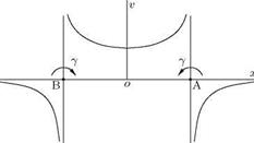
Thus u = 0, v = — 2aY/(x2 — a2). The plot of v against x is shown in Figure 5.52.

The curve is as per the equation v(x2 — a2) = —2aY, so that the asymptotes are the straight portions of Figure 5.52 go over into the asymptotes x ± a and thus the velocity of vortex A cannot be reached in Figure 5.52, although this is still one-quarter of the velocity at O.

5.17 Image of a Vortex in a Plane

For a vortex shown in Figure 5.51, because of symmetry there will not be any flux across yy’, the perpendicular bisector of AB. Thus yy’ can be regarded as a streamline and could therefore be replaced by a rigid boundary. Hence the motion due to a vortex at A in the presence of this boundary is the same as the motion that would result if the boundary were removed and an equal vortex of opposite rotation were placed at B. The vortex at B is called the image of the actual vortex at A with respect to the plane boundary and the complex potential is still given by Equation (5.78).