Category A PRACTICAL. APPROACH TO. ROBUSTNESS. ANALYSIS

Two mixed v upper bounds and a mixed v lower bound are proposed in this chapter.

1. A FIRST і/ UPPER BOUND

Let Д a mixed structured perturbation (see equation (1.26)). Remem­ber from chapter 5 that the sets V and Q of scaling matrices D and G are associated to Д:

Scaling matrix D must thus satisfy DA = AD.

Let Д = diag(AьДг), where Ді and Д2 are mixed structured per­turbations. Let mi the dimension of Дг. Scaling matrices Dt associated to perturbations Д* are introduced, with ДДг = Д Д■ D 1 and £>2 are then defined as:

so that D = .Di + D2 is a scaling matrix associated to perturbation Д. Proposition 1..1 presents a first mixed v upper bound (see subsection 2.1 of chapter 5 for the definition of the quantities A (A, B) and r)(A, B)).

PROPOSITION 1..1 (Ferreres and Fromion, 1997)

u(M) < л /max(0, inf + Di)M – Dl + j(GM – M*G),D2)) (8.3)

у Di,£>2iC

Remarks:

(i) The optimal values of scaling matrices Z>i, D2,G in Proposition 1..1 can be computed with recent methods for solving LMIs: see chapter 5 (subsection 2.1).

(/’/’) The v upper bound of (Fan and Tits, 1992) is recovered when the model perturbation A only contains full complex blocks.

(in) The classical p upper bound of (Fan et al., 1991) can be obtained in Proposition 1..1 by taking Ai empty, so that Di = 0.

It is possible under mild conditions to compute the exact value of v by computing recursively the exact value of p (see subsection 4.2 of chapter 1). Analogously, Proposition 1..2 claims that it is possible to compute the и upper bound of Proposition 1..1 by computing recursively the /і upper bound of (Fan et al., 1991).

PROPOSITION 1..2 (Ferreres and Fromion, 1997) Let:

IfvuB(M) < oo, then vub(M) is the unique limit of the fixed point iterationafc+i = h(otk), where h is defined as:

Local properties of a gain-scheduled control system can be analyzed with the p and и tools. Let в the vector of scheduling parameters: the

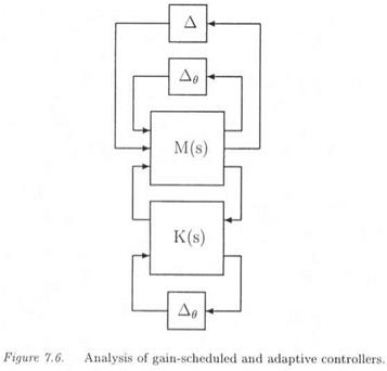
plant and controller can generally be expressed as LFTs involving a diag­onal matrix Ae, which contains possibly repeated parameters 0i(Ferreres et al., 1995). The augmented plant of Figure 7.6 is the closed loop ob­tained by connecting both LFTs. A structured perturbation Д is added to account for model uncertainties and performance blocks. Since the range of variation of the scheduling parameters is generally known a priori, a skewed /і problem is obtained, i. e. Ag is maintained inside its prescribed range of variation, while the size of Д is free.

An other skewed /л problem is obtained by introducing uncertainties 66i in the scheduling parameters 6f. the maximal allowable value of 86 is then computed, such that local stability or performance of the control system is guaranteed for all в belonging to a prespecified set. Note fi­nally that adaptive robust controllers can be analyzed in the same way (Ferreres et al., 1995).

It is briefly illustrated that the /x tool, the x sensitivities (see subsec­tion 4.5 of chapter 1) and the skewed ц tool can be combined in order to maximize the stability domain of the closed loop in the space of a structured model perturbation: see (Ferreres and M’Saad, 1996) for an application to a missile example.

For the sake of clarity, let a closed loop subject to just two paramet­ric uncertainties 5i and <52. Figure 7.4 shows the stability domain in the space of (5i and <52, which correspond to normalized uncertainties in the stability derivatives Nr and Щ of a missile (Ferreres and M’Saad, 1996). The zero point corresponds to the nominal closed loop system, which is by assumption asymptotically stable. /z analysis provides the

largest square in the parameter space, inside which closed loop stability is guaranteed. The и tool however provides the largest rectangle in the parameter space, inside which closed loop stability is guaranteed.

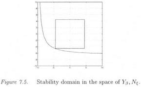
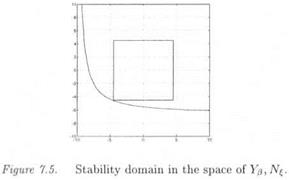
Nevertheless, the s. s.v. and the v measure can provide the same sta­bility domain, e. g. in the case of Figure 7.5 (81 and 82 now correspond to normalized uncertainties in the stability derivatives Y/3 and N ). In practice, p analysis is first applied. n sensitivities detect then whether the situation of Figure 7.4 or 7.5 is encountered. In the situation of Figure 7.4, the guaranteed domain of stability in the space of model uncertainties is further extended with the I’tool.

When applying fj, analysis to the standard interconnection structure M(s) — A(s), the s. s.v. m ( M(jw) ) is classically computed as a function of д using a frequency gridding, and the robustness margin is deduced as:

kmax = min l/fx&(M(jw)) (7.9)

UJ

However, especially in the case of flexible systems, narrow and high peaks may appear on the p, plot, so that only a prohibitively fine frequency gridding could find them (Freudenberg and Morton, 1992). An attract­ive solution in this case is to directly compute the maximal s. s.v. over the frequency range, or – more interestingly – over small frequency in­tervals (Ferreres and Fromion, 1997). As illustrated briefly below, this maximal s. s.v. can be computed as the solution of an augmented skewed p, problem.

The idea is to treat the frequency as an additional uncertainty. A possible solution is provided by the following Lemma: see (Ferreres and Fromion, 1997) and included references, see also (Doyle and Packard, 1987; Helmersson, 1995) for alternative methods.

LEMMA 3..1 Let (A, B,C, D) a minimal state-space model of the asymp­totically stable transfer matrix M(s). There exists a frequency uj Є [w, w and a perturbation Д satisfying det(I — M(jw)A) = 0 if and only if there exists an augmented perturbation A satisfying det(I — HA) = 0 with:

6w = ^ Є [0,1]

u> — W

6wlm 0 ‘

: 0 Д

: HflHX

jA~l A~lB

—jCA~l —CA~lB + D

0 ■ 0

Let цтах the maximal s. s.v. /j,(M(ju>)) over the frequency interval [tu, й>]. The following Proposition claims that the computation of цтах is a skewed /x problem: see also (Ferreres et al., 1996b) for an alternat­ive skewed Ц problem, in which the frequency is treated as a one-sided uncertainty [9].

Proposition 3..2

Umax = 1 /тіп(к / ЗД = diag(Sw, kA) with Su € [0,1], Д Є BA

and det(I – HA) = 0)

6w is thus maintained inside the interval [0,1], while the initial model uncertainty Д belongs to the expanded or shrunk ball кВА.

In the context of the robustness analysis of a flexible system, a first solution is thus to handle an augmented skewed /x problem in order to dir­ectly compute the maximal s. s.v. over a frequency interval. Nevertheless, we focus in this book on an alternative approach, which is computation­ally more efficient and which gives yet good results in practical examples: see chapter 10 and (Ferreres and Biannic, 1998a).

As an other example, consider the closed loop system of Figure 7.2. Ф represents a nonlinearity, whereas the LFT Fi(P(s), Д2) represents a

parametrically uncertain transfer matrix, i. e. N2 is a real model perturb­ation.

The Sinusoidal Input Describing Function (SIDF) N(X, w) is intro­duced for the nonlinearity 2> . For the sake of simplicity, N (N, N ) is defined for a SISO nonlinearity. The definition is however readily ex­tendible to the general case of a MIMO nonlinearity. A sinusoidal input u(t) = Xsin(u>t) is applied to Ф. The output of Ф, which is supposed to have odd symmetry, is written as:

y(t) — Rsin(wt) + Scos{wt) + e(t) (7.5)

where contains the super harmonic part of signal y(t). The SIDF is the complex gain:

N(X, w) = (7.6)

In the context of the first harmonic approximation, the signal e(t) is assumed to be filtered by the low-pass transfer matrix Fi(P(s),A2).

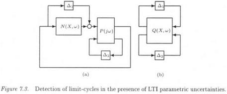
The MIMO nonlinearity N is now replaced by N(X,2) + Ді in the closed loop system of Figure 7.2 (see Figure 7.3.a). Roughly speaking, Ді is a block of neglected dynamics, which takes into account the super harmonic part e(t) of the signal y{t) (Katebi and Zhang, 1995; Ferreres and Fromion, 1998). N 1 is only known by the relation:

<т(Д) < а(Х, ш)

where n)N) n) is a known function of the magnitude X and frequency w of the limit-cycle.

Figure 7.3.a is then reshaped into Figure 7.3.b. A sufficient condition for the absence of limit-cycles in the nonlinear closed loop is given by:

a(Fl(Q(X, w),A2)) < —(7.8)
a(X, u))

As in the previous section, for given values of X and w, the problem consequently reduces to the issue of checking a small gain condition in the presence of a real model perturbation Д2: The aim is indeed to compute the maximal amount of parametric uncertainties, for which the sufficient condition (7.8) for the absence of limit-cycles remains satisfied.

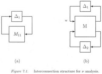
• Let the interconnection structure Ми— Ді of Figure 7.1.a, in which the full complex block Ді represents either a block of neglected dynamics, or a fictitious performance block (see section 4.4 of chapter 1). Мц contains the closed loop dynamics and the weighting function, the latter corresponding either to the template on the neglected dynamics, or to the performance requirement (i. e. the template on the closed loop transfer matrix of interest). In the rest of the subsection, the complex matrix Mi i typically represents the value of the transfer matrix Mn(s) at s = ju> (the same remark can be applied to the complex matrices M and Мц).

On the one hand, if A represents a block of neglected dynamics, this one is assumed to be maintained inside its unit ball (i. e. ст(Ді) < 1). The small gain theorem gives then a condition of stability of the interconnection structure, namely:

ct(Mu) < 1

On the other hand, if Ді represents a fictitious performance block, nom­inal performance is achieved if equation (7.1) is satisfied.

The transfer Fi(M, A2) between w and z (with Ді = 0 on Figure 7.1.b) can be computed as:

Fi(M, Д2) = Mu + Мі2Дг(/ — М22Д2) [8]Мгі

If W 1 represents a block of neglected dynamics which is to be maintained inside its unit ball, the small gain theorem gives then a condition of stability of the interconnection structure of Figure 7.1.b, namely ‘:

a(Ft(M, Д2))<1

On the other hand, if Ді represents a fictitious performance block, ro­bust performance (in the face of the model perturbation W2 ) is achieved if equation (7.4) is satisfied.

The issue is to find the maximal size of the structured model per­turbation Д2 which still satisfies, either the robust stability property in the presence of a given amount of neglected dynamics Ді, or the robust performance property (if Ді is a performance block). This maximal size is given by l/i>(M):

v(M) = l/min(k / ЭД2 Є кВА2 with M = Fi(M, Д2) anda(M) > 1)

The aim of this chapter is twofold. The first one is to detail some of the physical problems, which are solved in the rest of the book. The second one is to illustrate the usefulness of the skewed /л (i. e. v ) ap­proach for engineering problems. To this aim, a large class of important practical problems is considered, which requires the skewed ц tool rather than the classical ц tool. See also chapter 11 for the presentation of a specific problem, which uses an extension of the д and skewed ^ tools, namely the problem of computing a robust delay margin in the presence of model uncertainties.

Sections 1. and 2. give two examples, in which the problem of check­ing the robustness properties of a closed loop reduces to the problem of checking a small gain condition despite model uncertainties: as proved in chapter 8 (section 2.), this is a skewed ц problem involving an augmen­ted model uncertainty. See also chapter 11 (subsection 3.3) for an other example of problem which reduces to checking a small gain condition despite model uncertainties.

The difficult QFT problem of translating closed loop frequency do­main specifications into open loop specifications on the MIMO controller frequency response can also be solved in an approximate way with the skewed n tool. Here again, the problem reduces to the issue of checking a small gain condition despite a model uncertainty in the controller fre­quency response: see (Ferreres and LeGorrec, 1999) for further details (in a controller reduction context).

Three other examples of skewed /і problems are given in sections 3. to 5., namely the direct computation of the maximal s. s.v. over a frequency interval, the maximization of the domain of the allowable model uncer­tainties and the analysis of gain-scheduled or robust adaptive controllers.

As remarked in chapter 5, the mixed ц upper bounds of subsections

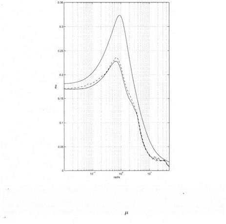
2.3 and 2.4 are equivalent. This can be checked on the example of Fig­ure 6.9, which corresponds to the robust stability problem (P4). The 4 plots represent the complex /x upper bound, the mixed / upper bound of subsection 2.4 and the mixed ц upper bound of subsection 2.3 (com­puted using the /x Analysis and Synthesis Toolbox and the LMI Control Toolbox). As expected, the results obtained with the 3 mixed /x upper bounds are essentially equivalent. The result provided by the LMI Con­trol Toolbox is globally more accurate than the one provided by the /x Analysis and Synthesis Toolbox. Nevertheless, it should be noted that the algorithm of the X Analysis and Synthesis Toolbox is designed in or­der to minimize the computational burden for large dimension problems. It is moreover possible to use various options, so as to achieve a balance between the accuracy of the result (i. e. the degree of optimality of the result) and the computational requirement.

Transport aircraft – robust stability inside a truncated sector (P5) – the

mixed /і upper bound by Fan et al is represented in solid line – the star represents the fi lower bound of section 3. of chapter 5.

Robust stability inside a truncated sector is now studied. The min­imal degree of stability (resp. the minimal damping ratio) is chosen as 0.4

(resp. 0.5). The nominal degree of stability (resp. the nominal damping ratio) is 0.7 (resp. 0.61). The results of Figure 6.8 are of the same type as those obtained in the previous subsection.

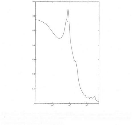
The maximal value of the mixed p upper bound is 0.648 at и = 0.79 rctd/s. The corresponding uncertainties in the stability derivat­ives are 10%/0.648 « 15%. The robust performance properties of the flight control system are thus quite satisfactory.

Transport aircraft – robust stability (P4) – the mixed a upper bound

by Fan et al is represented in dashed line (/i Analysis and Synthesis Toolbox) and solid line (LMI Control Toolbox) – the mixed fi upper bound by Safonov and Lee is

represented in dash-dotted line – the complex

line.

The star on Figure 6.8 represents the ^ lower bound of section 3. of chapter 5. When computing this p lower bound as a function of frequency, two different peaks are obtained: the first one is 0.579 at u> = 0 (the corresponding value of the p upper bound is 0.58 at w = 0), while the second one is 0.564 at u> = 0.76 rad/s. The lower bound of
the maximal s. s.v. over the frequency range is thus obtained as 0.579 at o> = 0, while the upper bound is obtained as 0.648 at ш = 0.79 rad/s. The gap between the bounds of the maximal s. s.v. over the frequency range is thus about 10.6 %, which is quite reasonable.

Transport aircraft – robust stability (P4) – the mixed /1 upper bound by

Fan et al is represented in solid line – the star (resp. the circle) represents the u. lower bound of section 3. of chapter 5 (resp. the one by (Magni and Doll, 1997)).

With reference to chapter 2, the rigid aircraft of subsection 1.1 is considered, and the robustness properties of the static output feedback controller of subsection 1.2 are studied. The case of the flexible aircraft will be considered in chapter 10. The model perturbation consequently contains 14 real non repeated scalars, corresponding to uncertainties in the stability derivatives. The weights in these stability derivatives are chosen as 10 %. Because of the large number of uncertainties, only polynomial time methods can be applied to this problem. See table 6.1 for a summary of numerical results.

1.1 ROBUST STABILITY (P4)

Figure 6.7 presents the mixed /supper bound as a function of frequency ш. The maximal value is 0.229 at r = 0.70 rad/s. The corresponding

uncertainties in the stability derivatives are 10%/0.229 « 43.5%. The robust stability properties of the flight control system are thus very good.

The star on Figure 6.7 represents the ц lower bound of section 3. of chapter 5 (method # 1 – see chapter 10 for a comparison of methods #1 to #3 in the case of the flexible aircraft). This /і lower bound is obtained as 0.184 at ш = 0.63 rad/s. The gap between the bounds of the maximal s. s.v. over the frequency range is about 19 %, which is acceptable. The circle on this same Figure represents the /і lower bound by (Magni and Do 11, 1997), which is obtained as 0.177 atw = 0.63 rad/s. The two lower bounds give thus a rather equivalent result in the case of this example.