Category COMPUTATIONAL AEROACOUSTICS

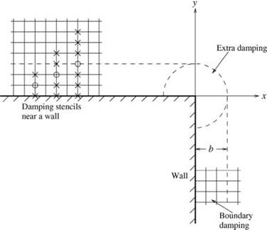
A surface of discontinuity such as a wall is a potential source of spurious waves. Thus, it is important to incorporate artificial selective damping near such a surface to suppress the generation of these waves.

Near a horizontal wall, there is not enough room for a 7-point central damping stencil in the vertical direction for mesh points in the two rows adjacent to the wall (see Figure 7.7). Only a smaller symmetric stencil can fit in the limited space. The following are stencil coefficients for 5-point and 3-point stencils that have been used extensively with satisfactory results.

5-Point Damping Stencil

d0 = 0.375 dx = d—1 = —0.25 d2 = d—2 = 0.0625.

3-Point Damping Stencil

d0 = 0.5

dx = d—1 = —0.25.

The damping curves for these stencils are shown in Figure 7.4. These smaller damping stencils impose a nonnegligible damping on the long waves. They should not be used as general damping stencils over the entire computational domain.

Experience indicates that, when used only near a wall or at the outside boundary of a computational domain, they do not cause excessive damping to the physical solution.

For general background damping, the use of an inverse mesh Reynolds num­ber, Яд1, of 0.05 or slightly less has been found to be satisfactory. The amount of damping is sufficient to remove spurious short waves in most problems. For viscous fluid, additional damping near a wall, especially at a sharp corner (see Figure 7.7), is often necessary. To impose extra damping, a simple but effective way is to use a Gaussian distribution of Яд1 in the direction normal to the wall. The peak value of the Gaussian is at the wall. A good choice of the half-width of the Gaussian is three or four mesh spacings. For instance, along the wall y = 0 in Figure 7.7, an additional inverse mesh Reynolds number distribution of the following form,

Яд1 = 0.15c-(ln2)(H(y), (7.26)

where H(y) is the unit step function, may be incorporated into the artificial selective damping terms of the computation scheme. The highest value of Яд1 at the wall may be larger than 0.1 as indicated above. A similar distribution of inverse mesh Reynolds number distribution may also be imposed adjacent to the wall at x = 0.

At a sharp corner, as shown in Figure 7.7, large amount of artificial selective damping is required to stabilize the computation. This may be implemented by using an inverse mesh Reynolds number distribution at the corner point in the form of a multidimensional Gaussian function,

ЯД = 0.3e~ . (7.27)

At the present time, there are no formal guidelines to setting the amplitude of the Gaussian function at the corner point. This value has to be adjusted in each problem until a satisfactory value is selected.

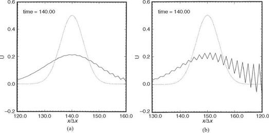
Now the phenomenon of “numerical instability” caused by excessive artificial damp­ing is investigated. Suppose the solution of Eq. (7.21) is again computed with the initial condition (7.22), but with even larger damping, say RA1 = 15. Figure 7.6 shows the computed result as time increases. At t = 140, Figure 7.6a shows the onset of numerical instability. The instability wave has a wave length of about two mesh spacings or a Ax = n. This is grid-to-grid oscillation. At t = 150, Figure 7.6b shows that the numerical instability has grown in amplitude rapidly. At t = 400, Figure 7.6c shows that the instability completely overwhelms the numerical solution.

It is not difficult to understand why excessive artificial damping can lead to numerical instability. For this purpose, consider the Fourier-Laplace transform of Eq. (7.21). The transform of the finite difference equation is

_ _ 1 –

— i ши + i au =—- D (aAx)u.

ra

Thus, the dispersion relation is

ш = a——— D (aAx).

Ra

Consider grid-to-grid oscillation instability wave with aAx = n. It is to be noted that a(n) = 0.0 (see Figure 2.3) and D (n) = 1.0 (see normalization condition (7.18)). Therefore, for this wave, dispersion relation (7.24) reduces to

-л – At

ш At = —i—. Ra

Figure 3.2 gives the stable region in the complex «At-plane. Along the imagi­nary axis, the four-time level DRP marching scheme is stable if Im(«At) > —0.29. Therefore, there will be numerical instability unless At/RA = 0.29. In the numer­ical example, the time step At is 0.02 and 1/RA = 15 so that At/RA = 0.3. Thus, the numerical scheme is outside the region of stability, and one should not be too surprised to see numerical instability.

Consider again the one-dimensional convective wave equation in dimensionless form as follows:

d U d U

+ = 0 —ж < x < ж.

dt dx

Suppose Eq. (7.20) is discretized according to the DRP scheme with the addition of artificial selective damping terms. The discretized equations are

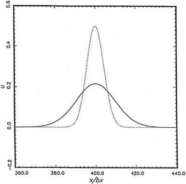
For the stated purpose, RA1 is taken to be equal to 5. This is about 15 times more damping than what was used in the previous example. Suppose the initial condition is

In Chapter 2, it was demonstrated that the 7-point stencil DRP scheme can provide an almost error-free solution for this initial value problem when there is no artificial damping. Figure 7.5 shows the computed result at t = 400 by using a damping stencil with a = 0.3 n and At = 0.02. By comparing the computed waveform and the exact solution, it is clear that there is an overall reduction in the wave amplitude. However, at points farther away from the center of the pulse, the wave amplitude has actually increased, as if the pulse has diffused outward on both sides. This is a very unexpected phenomenon.

The cause of this apparent diffusion effect is subtle but can be understood by viewing the damping process in wave number space. Since the Fourier transform of a Gaussian function is also a Gaussian function, the initial pulse is also a concentrated pulse around a Ax = 0 in the wave number space. Now in time, the artificial selective damping terms gradually reduce the amplitude of the pulse in the wave number space, but not evenly. By design, there is no reduction at zero wave number. The reduction increases with wave number. Because of this, the half-width of the pulse in wave number space is reduced over time. The maximum height that occurs at a Ax = 0, nevertheless, remains the same. The waveform in the physical space is the Fourier inverse transform of the waveform in the wave number space. With a narrower pulse, as time increases, the physical waveform spreads out according to the Inverse Spreading Theorem of Fourier transform. Thus, artificial selective damping has the unintended side effect of inducing artificial viscous diffusion.

It was shown in previous sections that, by adding artificial selective damping to a finite difference equation, the short waves are eliminated. However, if too much
damping is used, there are also negative effects. Excessive selective damping can basically result in “artificial viscous diffusion” and “numerical instability.” Here, the phenomenon of “artificial viscous diffusion” will be discussed first.

The a = 0.3 n 7-point damping stencil with damping function shown in Figure 7.2 is primarily designed for problems with discontinuities or shocks. Because of the steep gradients involved, strong damping over a wide band of wave numbers is necessary. But even in problems for which the solutions are shock and discontinuity free, short spurious waves are often generated. Wall boundaries, mesh size change interfaces and regions with steep gradients are potential sources of short waves. For this reason, it is a good practice to add a small amount of background artificial selective damping to a computation. Also because of the need to use backward difference stencils at the boundary region of a computation domain, the numerical solution is subjected to weak numerical instability. These instabilities usually manifest themselves in the form of grid-to-grid oscillations with very gradual increase in amplitude. This type of weak instability can easily be suppressed by the addition of artificial selective damping.

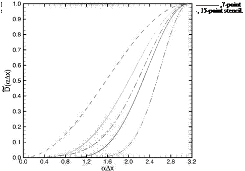
For general background damping for which only short waves need to be removed, the following a = 0.2 n 7-point damping stencil is recommended. The stencil coefficients are as follows:

7-Point Damping Stencil (a = 0.2n)

d0 = 0.2873928425 d4 = d_! = -0.2261469518 d2 = d_2 = 0.1063035788 d3 = d_3 = -0.0238530482

The damping function of this damping stencil is shown in Figure 7.4.

When very high resolution is required, a 15-point stencil DRP scheme may be used. The following is a set of damping coefficients for such a stencil.

15-Point Damping Stencil

d0 = 0.2042241813072920 d1 = d_1 = -0.1799016298200503 d2 = d_2 = 0.1224349282118140 d3 = d_3 = -6.3456279827554890E – 02 d4 = d_4 = 2.4341225689340974E – 02 d5 = d_5 = -6.5519987489327603E – 03 d6 = d_6 = 1.1117554451990776E – 03 d7 = d_7 = -9.0091603462069583E – 05

The damping curve is shown in Figure 7.4.

To illustrate the effectiveness of artificial selective damping, consider again the simple wave problem with discontinuous initial condition. On incorporating artificial selective damping to the DRP scheme, the finite difference equations are

3

Ul = T ^ ^ bjEt

j=0

3

рГГ) = pf + At Ь^П_j)

j=0

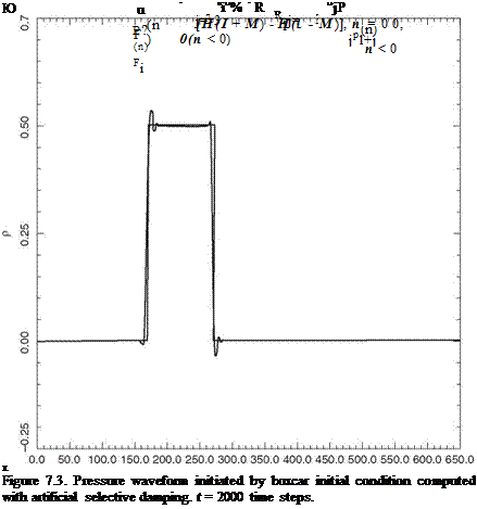where Ra = a0kx/v is the artificial mesh Reynolds number. In the numerical simu­lation below Ra1 is given the value of 0.3.

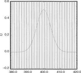
In the course of computing the numerical solution of Eq. (7.19), it is noticed that the short waves corresponding to grid-to-grid oscillations that are subjected to most intense damping are damped out almost immediately after they are generated. The damping for the spurious waves with longer wavelengths is smaller. Their presence in the numerical solution can still be seen after 200 time steps. At t = 500At, they, too, are almost completely eliminated. Figure 7.3 shows the calculated pressure waveform at t = 2000At. Essentially all the spurious waves, except for two spikes, have been damped out. The computed solution is now a reasonably good approximation of the exact boxcar solution. Of course, the finite difference solution is not perfect. It does not faithfully reproduce the sharp discontinuities. Each discontinuity is spread over

a distance of about 5 to 6 mesh spacings. This is closed to the minimum wavelength that the scheme can resolve.

Suppose a damping term, D(x), is added to the right side of the momentum equation of the linearized Euler equations in dimensional form as follows:

d u 1 d p

—— 1—– –

dt p0 дX

Let the spatial derivative be approximated by the 7-point stencil DRP scheme. The discretized form of Eq. (7.10) is

It will now be assumed that De is proportional to the values of ut within the stencil. Let dj be the weight coefficients. Eq. (7.11) may be written as

where v is the artificial kinematic viscosity. v/(Ax)2 [4] has the dimension of (time)-1, so that dj’s are pure numbers. Now djs are to be chosen so that the artificial damping would be effective mainly for high wave number or short waves.

The Fourier transform of the generalized form of Eq. (7.12) is,

di v,

d + ”’ = "<Arf2D (aAx)u (7-13)

where

3

D (aAx) =Y^ djeijaAx j=-3

On ignoring the terms not shown in Eq. (7.13), the solution is,

Since D (a Ax) depends on the wave number, the damping will vary with wave number. It is desirable for D to be zero, or small for small a Ax, but large for large a Ax. This can be done by choosing dj’s appropriately. But one must be careful to make sure that the damping term would not cause undamping or numerical instability. The purposes of the following three conditions that are to be imposed on D are self-evident.

1. D (a Ax) should be a positive even function of a Ax. The even function condition is ensured by setting dj = dj. Thus,

3

D (a Ax) = d0 + 2 ^2 dj cos( j a Ax). (7.16)

j=-3

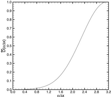
For example, the coefficients of a very useful damping curve for problems involving discontinuous solution are (a = 0.3п, в = 0.65n) as follows

d0 = 0.3217949913 dx = d_! = -0.2328759104 d2 = d_2 = 0.08910250435 d3 = d_3 = -0.01712408960

A plot of D versus a Ax for this choice is shown in Figure 7.2.

The short waves are numerical contaminants of a computed solution. To improve the quality of a numerical solution, it is imperative that the short waves be automatically removed from the computation as soon as they are generated. A way to remove short waves is to add artificial selective damping terms to the finite difference equations.

For this method to be acceptable, the damping terms must selectively damp out the short waves and have minimal effect on the long waves.

It was pointed out previously that when a central finite difference scheme was used to approximate the spatial derivative, the wave number of the finite difference scheme a was related to the actual wave number a. Figure 2.1 shows a typical relationship between a Ax and a Ax. Earlier, it was also suggested that the wave spectrum might be divided into two parts; the long waves (waves for which a ~ a ) and the short waves (waves for which a is very different from a). The long waves behave like the corresponding wave component of the exact solution. In this chapter, attention is focused on the short waves.

7.1 The Short Waves

To fix ideas, consider the initial value problem associated with the linearized Euler equations in one space dimension without mean flow. The same dimensionless vari­able as in Section 6.4 is used. The dimensionless linearized momentum and energy equations are as follows:

where M is a large positive number and H(x) is the unit step function. The wave num­ber spectrum of Eq. (7.6) extends well beyond the range – п < a < n. A considerable fraction of the spectrum falls in the short wave range. This offers an excellent exam­ple on the wave propagation characteristics of the short waves of finite difference schemes. From Eq. (7.5), the exact solution is

1 1

p(x, t) = 2 [H(x – t + M) – H(x – t – M)] + 2 [H(x +1 + M) – H(x +1 – M)].

(7.7)

It is of interest to find out what happens when the problem is solved by the 7-point stencil dispersion-relation-preserving (DRP) scheme. On discretizing Eqs. (7.1) and (7.2) according to the DRP scheme, the resulting finite difference equations are

3

E"’ = – £ ajP“j

j=-3

3

F“ = – £ aUH,

j=-3

3

u("+1) = uf + AtJ2biEf – j)

j=0

3

рГ1’=p»+1>+a, j2i>,f;"-h.

j=0

The initial conditions corresponding to Eqs. (7.3) and (7.6) are

U" = 0, " < 0

(") = 1H(l + M) – H(l – M), " = 0

Pl {0, " < 0

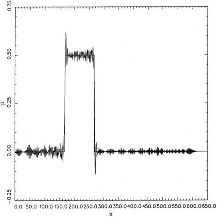
Figure 7.1 shows the numerical solution with the boxcar initial condition

(M = 50). As can be seen, the solution is badly contaminated by short waves. The lead waves are the grid-to-grid oscillatory waves. The envelope of the amplitude of the short waves oscillates spatially (giving the appearance of lumps of waves). The longer dispersive waves are trailing the main pulse solution.

This example clearly shows that short waves are pollutants of numerical solu­tions. They can be generated by discontinuous initial or boundary conditions. To render numerical solutions acceptable, a way must be found to suppress or eliminate the short waves without interfering with the long waves.

When curved surfaces are involved in a computation, very often a body-fitted grid is used. It will now be assumed that the computation grid is on a set of orthogonal

Figure 6.17. Orthogonal curvilinear co­ordinates (f, n, Z) forming a body-fitted curved surface.

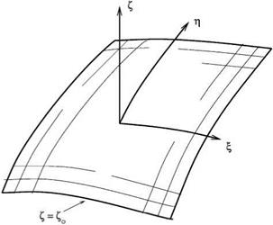curvilinear coordinates f (x, y, z), n(x, y, z), and Z (x, y, z). The coordinate system is orthogonal, meaning that

Vf ■ Vn = Vn ■ VZ = VZ ■ Vf = 0. (6.26)

Without the loss of generality, the curved boundary surface is taken to be on the Z = Zo coordinate surface as shown in Figure 6.17. The normal to the surface is in the direction of VZ.

The Euler equation in curvilinear coordinates (f, n, Z) is given by Eq. (5.61).Let U = v ■ Vf, V = v ■ Vn, W = v ■ VZ (the contravariant velocity components), i. e.,

n 9f 9f 9f

dx 9y 9 z

9n 9n 9n

V = u + v + w dx dy 9 z

w 9Z 9Z 9Z

W = u + v + w . dx dy 9 z

The momentum equation in the Z direction may be found by multiplying the second equation of (5.61) by Zx, the third equation by Zy, and the fourth equation by Zz (subscript denotes partial derivatives), then summing up the three equations. On being written out in full, the equation is as follows:

For inviscid flow, the wall boundary condition is W = 0on Z = Zo (the solid surface). To enforce the wall boundary condition, it is recommended to include a set of ghost points on the surface Z = Zo – AZ as shown in Figure 6.18. At each ghost point, a ghost value of p is included in the computation. The computation is carried out in the (f, n, Z) space. It is similar to computation in a Cartesian coordinate system.

Figure 6.18. Computational grid and ghost points near a solid wall in a com­putational domain.

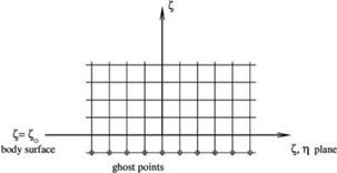
For all mesh points inside the computation domain, the discretized form of Eq. (5.61) is used. For all flow variables, with the exception of p, backward difference stencils for d/dz are implemented for points in the boundary region. This is to keep the stencil points inside the computational domain. For 9p/dz, the stencils are extended to the ghost points. For mesh points lying on the solid surface z = Zo, instead of the second, third, and fourth equation of (5.61), Eq. (6.28) and two of the three equations are used. Let (l, m, n) be the spatial indices in the Z, n, and z directions, respectively, and z = zo corresponds to n = N, the discretized form of Eq. (6.28) at n = N, taking into account that the boundary condition W = 0 at z = zo, is as follows:

where superscript k is the time level.

The ghost value of pressure, pf}m N—1, may now be calculated by Eq. (6.29). The explicit formula is as follows:

p(k) =__ 1 a51 „0

pl, m,N—1 = a51 U1 pl

a—1 j=0

With the ghost value of p found, the computation can proceed as in the case of a flat wall.

For viscous flows, the full Navier-Stokes equation must be used in the computa­tion. The boundary conditions on the curved solid surface are the no-slip conditions. Because the stress terms are fairly complicated in curvilinear coordinates, the use of ghost values of shear stresses to enforce the no-slip boundary conditions would require a good deal of effort. A less complicated approach is to set (u, v, w) to zero on z = Z0 (n = N). To avoid the computation becoming an overdetermined system, the three momentum equations will not be used for mesh points right at the solid surface. For density p and pressure p on the solid surface, they are to be computed by means of the continuity and energy equations. Although this approach is a bit less accurate, this way of treating the curved wall boundary condition has been found to be quite efficient, easy to implement, and offers reasonably accurate results.

EXERCISES

6.1. Consider solving the one-dimensional wave equation

d 2U 2d2U

dt2 C dx2

in a finite domain. The equation has two solutions:

u = F(x – ct) + G(x + ct),

where F and G are arbitrary functions. The solution F (x – ct) represents a wave propagating to the right, and the solution G(x + ct) represents a wave propagating to the left.

Develop a radiation boundary condition for the right and the left boundary of the computation domain.

6.2. For problems with spherical symmetry, it is advantageous to use spherical coor­dinates (R, в, ф). The linearized Euler equations in spherical coordinates for prob­lems with spherical symmetry are (9/9в = 0, Э/Эф = 0) as follows:

— + 1 dp = 0

91 p0 d R

where «0 = yp0/p0. The general solution of (3) is

_ F(R – a0t) + G(R + a0t)

P _ R + R ‘ ()

F and G are arbitrary functions. Derive a radiation boundary condition for p at large R. In solving the system of equations (1) and (2) a boundary condition for v is also needed. Derive a boundary condition for v.

6.3. Use dimensionless variables with respect to the following scales:

Ax _

aO (ambient sound speed) _ Ax

a

pO _ density scale
P^aO _ pressure scale

The linearized two-dimensional Euler equations on a uniform mean flow are to be solved

9 U 9 E 9 F

dt dx 9y

where

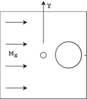
Mx and My are constant mean flow Mach number in the x and y directions, respec­tively. Use a computation domain -100 < x < 100, -100 < y < 100 embedded in free space.

(a) Let Mx = 0.5, My = 0. Solve the initial value problem, t = 0.

– <ln2>(^У

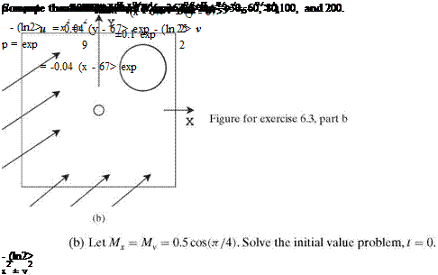
■- (ln2> (Цгу + 0.1 exp [- (ln2><K^6^У

Note: The mean flow is in the direction of the diagonal of the computational domain. Compute the distributions of p, p, and u at t = 60, 80, 100, 200, and 600.

6.4. The exact solution of the initial value problem of the diffusion equation,

d u f 9 2u 9 2uл

9t 9 x2 + 9 y2,

(x2+y2 >

-(ln2> b-

Suppose one is interested to find the solution computationally by using the DRP scheme. Let Ax = Ay be the length scale and (Ax)2/к be the time scale, so that the nondimensional diffusion equation becomes

du d2U d 2U

dt dx2 dy2

t = 0

To solve this problem computationally in a finite domain requires numerical bound­ary conditions. For diffusion equations, the asymptotic solution is not useful for constructing a numerical boundary condition.

It is observed, because of the diffusive nature of the solution, that the solution at a point depends mainly on the solution on the side closer to the source. For this reason, it is recommended that one use backward difference stencils at mesh points close to the exterior boundaries of the computation domain. No other spe­cific boundary conditions at the outer boundaries of the computation domain is needed.

Compute the solution on a 100 x 100 mesh with b = 3. Compare your numerical solution with the exact solution by plotting u(x, 0, t) at t = 20, 40, 80,160, 300. See Appendix D for helpful suggestions.

6.5.

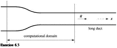Consider one-dimensional flow and acoustics in a nozzle attached to a long duct of uniform cross section as shown. For calculating the flow and acoustic waves in the nozzle, it is decided to use a computation domain encompassing the variable area part of the nozzle. The right boundary of the computation domain is in the uniform duct. A small-amplitude sound wave of angular frequency ы propagates from the uniform duct into the nozzle region. Part of this wave is transmitted through the nozzle throat and a part of it is reflected back into the uniform duct.

Let u, p, and p be the mean flow in the uniform area duct. The linearized gov­erning equations in the duct are the continuity, momentum, and energy equations.

The upstream propagating acoustic wave in the uniform duct is given by

(4)

where a = (yp/p)1/2 is the sound speed. F is a known function.

Develop a set of outflow boundary conditions for use on the right side of the computation domain.

If the left side of the nozzle is attached to another long uniform duct, hot spots in the form of entropy waves are convected downstream by the mean flow into the nozzle. The entropy wave solution may be written as

where U is the local mean flow velocity of the uniform duct and H is a known function characterizing the density (temperature) distribution.

Develop a set of inflow boundary conditions for use on the left side of the computation domain.

6.6. Consider acoustic radiation from an oscillating circular piston in a wall as shown below.

Let the radius of piston be R and the velocity of piston be u = є sin(nt/5). Use a computational domain 0 < x < 100, 0 < r < 100. The wall and the piston are at x = 0. The cylindrical coordinate system is centered at the center of the piston. With axisymmetry, the dimensionless linearized Euler equation is

The initial conditions are

t = 0, p = u = v = p = 0.

Compute the time harmonic pressure distribution at the beginning, 1 /4,1 /2, and 3/4 of a period of piston oscillation.

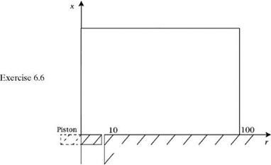Let e = 10 4, R = 10, ю = n/5. The exact solutions is

TO

6.7. A spherically symmetric acoustic pulse is initiated at time t = 0 by a small – amplitude pressure pulse of the following form:

p = p = ee – (ln2)[(x2+y2+z2 )/b2]

in a static environment. Here, the length scale is Ax = Ay = Az, the velocity scale is a0 (the speed of sound), the time scale is Ax/a0, the density scale is p0 (the mean gas density), and the pressure scale is p0a0. Compute the solution by solving the three­dimensional Euler equations in Cartesian coordinates. Take e = 10-4 and b = 3.

Let R = (x2 + y2 + z2)1/2 be the radial distance. The exact linearized solution is

p = e R – 1 e-(ln2)[(R-t)/b]2 + R + 1 e-(ln2)[(R+t)/b]2

p 2R 2R

Note: A computer code for this problem is provided in Appendix G.