Category COMPUTATIONAL AEROACOUSTICS

The optimized central difference scheme for approximating spatial derivatives introduced in Chapter 2 will give rise to ghost points (points outside the compu­tational domain) at the boundaries of the computational domain. For a 7-point stencil, 3 ghost points are created. To advance the entire computation to the next time level, a way to calculate the unknowns at the ghost points must be speci­fied. Here, it is suggested that this is done using the radiation or outflow boundary conditions.

Figure 6.1 shows the upper right-hand corner of a computation domain. Three columns or rows of ghost points are added to form a boundary region surrounding the original computation domain. For grid points inside and on the boundary of the interior region, Eqs. (5.28) and (5.29) discretized according to the DRP scheme are used to advance the calculation of the unknowns to the next time level. In the bound­ary region it will be assumed that the solution is made up of outgoing disturbances satisfying the radiation or outflow boundary conditions of Eq. (6.2) or Eq. (6.13). The time derivatives of these equations are discretized in the same manner as described in Chapter 3. These equations are to be used to advance the solution in time. Now, all the variables in the boundary region as well as in the interior regions can be advanced in time simultaneously. To approximate spatial derivatives, symmetric spatial stencils are not always possible for points in the boundary region. The opti­mized backward difference stencils of Chapter 2 are to be used whenever necessary. An example of such backward difference stencils is illustrated by that of the corner point B in Figure 6.1. In the boundary region, the domain of dependence of the outgoing waves is consistent with that of the backward difference approximations.

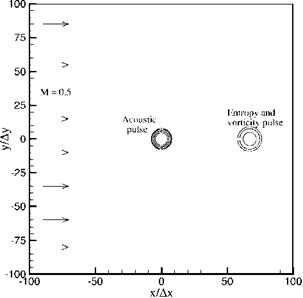
Figure 6.2. Computational plane show­ing a uniform mean flow of Mach 0.5 and initial acoustic, vorticity, and entropy disturbances.

Unlike the use of unsymmetric stencils at interior points where waves may propagate in any direction, no numerical instability would be created unless there are strong reflections of waves back into the interior.

At boundaries where there are only outgoing acoustic waves, the solution is given by an asymptotic solution (5.25) as follows:

where V(e) = a0[M cos в + (1 – M2 sin2 в)1/2]. The subscript ‘a’ in (pa, ua, va, pa) in Eq. (6.1) indicates that the disturbances are associated with the acoustic waves alone. By taking the time t and r derivatives of formula (6.1), it is straightforward to find that for arbitrary function F the acoustic disturbances satisfy the following equations:

P

/ 1 д д й

V (в) дt дГ 2r/ V

p

Eq. (6.2) provides a set of radiation boundary conditions.

where the explicit form of (pa, ua, va, pa) may be found in Eq. (6.1). The functions X, f, and F are entirely arbitrary. It is observed that the total pressure fluctuation comes only from the acoustic component of the outgoing disturbances. Thus, the appropriate outflow boundary condition for p is the same as that of Eq. (6.2). On writing out Cartesian coordinates in two dimensions, it is
d p.9 p p + cos в — + sin в — + ^~ d x dy 2r
(6.4)
0,
where в is the angular coordinate of the boundary point. By differentiating the expression for p in Eq. (6.3) with respect to t and x, the following equation is found:
dp dp dp dp„ — + U0—— = — + u0—. 91 0 dx 91 0 dx
(6.5)
But pa = pa/a2 = p/a0 andp is known from Eq. (6.4). By eliminating pa, the outflow boundary condition for p becomes
du 9 u 1 9 p 91 0 dx p0 dx 9 v 9 v 1 9 p dt ^ U° 9x p0 9y ’ In summary, the outflow boundary conditions are as follows:
(6.11) (6.12)
(6.13)

A computational domain is inevitably finite. For open domain problems, this auto­matically creates a set of artificial exterior boundaries. There are two basic reasons why exterior boundary conditions are needed at the artificial boundaries. First, exte­rior boundary conditions must reproduce the effects the outside world exerts on the flow inside the computation domain. Since only the computed results inside the computational domain are known, in general, it is not possible to know the outside influence. For this reason, a computation domain is often taken as large as possi­ble so that all sources are inside. This will minimize any external influence that is unaccounted for.

Another reason for imposing exterior boundary conditions is to avoid the reflec­tion of outgoing disturbances back into the computational domain and thus contam­inate the computed solution. One way to avoid reflection is to construct boundary conditions in such a way to allow the smooth exit of all disturbances.

In this chapter, it will be assumed that there is little external influence and there are no incoming disturbances. Issues of external influence and incoming entropy, vorticity, or acoustic waves will be considered in later chapters.

As discussed previously, the linearized Euler equations support three types of waves. Two types of these waves, namely, the entropy and vorticity waves, are convected downstream by the mean flow. The acoustic waves, however, propagate and radiate out in all directions if the mean flow is subsonic. Thus, at a subsonic inflow region, the outgoing waves consist of acoustic waves alone. In the outflow region, the outgoing disturbances now comprise of all three types of waves. As a result, it is prudent to develop separate inflow and outflow boundary conditions.

Many aeroacoustics problems involve solid surfaces. To specify the presence of these surfaces, the no-slip boundary conditions are imposed if the fluid is viscous. On the other hand, if the fluid is inviscid, the no-through flow boundary condition is to be used. How to impose these physical boundary conditions on a high-order finite difference computation without creating excessive spurious short waves is one of the main topics of this chapter.

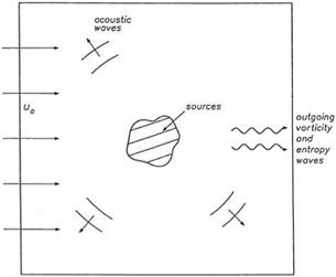
Now, consider an exterior problem involving a uniform flow of velocity u0 and sound speed a0 past some arbitrary acoustic, vorticity, and entropy sources as shown in Figure 5.1. It will be assumed that the boundaries of the computation domain are quite far from the sources. From the analysis of Chapter 5, it is clear that outflow

boundary conditions are needed on the right side of the computational domain with outgoing disturbances formed by a superposition of acoustic, entropy, and vorticity waves. On the other hand, at the top and bottom boundaries, as well as the left inflow boundary of the computational domain, the outgoing disturbances are acoustic waves only. Now, the exterior boundaries are far from the sources, the outgoing waves in the regions close to these boundaries are, therefore, given by the asymptotic solutions of the discretized form of the governing partial differential equations. It will now be assumed that the DRP scheme is used for time-marching computation. However, in the resolved wave number range, the DRP scheme and the original partial differential equations have (almost) identical dispersion relations and asymptotic solutions. These solutions are given by Eqs. (5.14), (5.16a, b), and (5.25). A set of radiation and outflow boundary conditions will now be constructed based on these asymptotic solutions.

Most practical computations are often not carried out in Cartesian coordinates. Instead, the actual computations usually are done on a set of body-fitted curvilinear coordinates. Thus, the space of the curvilinear coordinate system forms the com­putation domain. In other words, the governing equations, written in curvilinear coordinates, will be discretized and computed. It will be shown that, if the optimized spatial and temporal discretization method developed in Chapters 2 and 3 are used, then the discretized equations retain the DRP property.

The three-dimensional compressible Euler equations for a perfect gas in Carte­sian coordinates may be written as

d u 9 u „ 9 u

—– + A—— + B—

dt dx dy

where

Now, let f (x, y, z), n(x, y, z), and Z (x, y, z) be a set of curvilinear coordinates. This set of coordinates will be used for discretizing the Euler equations and for computing the solution. A simple change of variables by means of the chain rule transforms Eq. (5.60) into an equation with (f, n, Z) as independent variables in the following form:

where

A = df A+df B + df c

dx dy dz

B = —a + A B + Ac

dx dy dz

c = A – A + a B + A c.

dx dy dz

Suppose the Fourier-Laplace transform of a function/(f, n, Z, t) is /(а, в, Y,«) and that of

(5.62)

By means of convolution interal (5.62), the Fourier-Laplace transform of the Euler equation (5.6i) may be written as follows:

+ i^B(a — ai, в — во Y — Yi, a — ai) + i’YiC(a — ai, в — во Y — Yi, a — ai)] x ii(ai, в1, Yi, ai) dai dв1 dYi dai.

Now, for the purpose of computation, let Eq. (5.6i) be discretized in the (f, n, Z) spacing using the 7-point stencil optimized scheme and the four-level time march­ing algorithm developed in Chapters 2 and 3. The discretized equations are as follows:

j=0

The Fourier-Laplace transforms of the discretized Eqs. (5.64) and (5.65) are

— ai, в — ві, Y — Уі, « — «і) + i У(Уі)C(a — аі, в — ві, Y — Уі, « — «і)]

x й(аі, ві, Y!, «і) da1 dв1 dY1 й«і – (5.67)

Upon eliminating Ё from Eqs. (5.66) and (5.67), the Fourier-Laplace transform of the discretized solution is given by

аі, в — ві, Y — Уі, « — «і)

+ i в(ві)B(a — аі, в — ві, Y — Уі, « — «і)•

+ i У(Уі)C(a — аі, в — ві, Y — Уі,« — «і)] x й(аі, ві, Y^ «і) dax dв1 dY1 d«v (5.68)

By comparing Eqs. (5.63) and (5.68), it becomes clear that, if the discretized solution is restricted to the range for which а(а) = а, в(в) = в, Y(y) = Y, and «(«) = «, the equations are identical. Thus, the discretized Eqs. (5.64) and (5.65) are DRP in the sense that their Fourier-Laplace transforms are formally the same as the exact solution of Euler equations.

EXERCISES

5.1. The propagation of electromagnetic waves is governed by the Maxwell equa­tions:

where Ё and B are the electric and magnetic fields and д and є are material constants. Now, look for plane wave solutions in the following form:

Ё = e E/(k’x—«(), (5)

where e is a constant unit vector characterizing the direction of the electric field. E0 is the amplitude and k = aex + в ey + у ez, where ex, ey, ez are the unit vectors in the

x, y, and z directions, is the wave vector and ш is the angular frequency. Eqs. (2) and (4) are satisfied automatically if the magnetic field is given by

c

B = – (k x E). (6)

ш

Substitution of (5) and (6) into (1) and (3) leads to

шілє~ ci /і ^

—- e = — k x (k x e)

c ш

Є ■ k = 0.

(Note: Eqs. (7) and (8) can also be obtained by taking the Fourier-Laplace transform of Eqs. (1) to (4). In this case, the transform variables are (а, в, у, ш)).

If Є = f Єх+ + пЄу + Zez is the solution of Eq. (7), then Eq. (8) is automatically satisfied. By writing Eq. (7) in a matrix form for the unknowns (f, n, Z), the disper­sion relations of electromagnetic waves are given by setting the determinant of the coefficient matrix to zero.

Discretize the Maxwell equations according to the DRP scheme. Show that the discretized equation formally preserves the dispersion relation of the electromag­netic waves; i. e., ш replaces ш, (а, в, у) replaces (а, в, у), respectively.

5.2. Consider solving the convective equation

d u d u

——- + c— = 0

dt dx

computationally by using central difference approximation. Suppose we use differ­ent size stencils; e. g., N = 7, 9, 11 etc. Assume that the same time marching scheme is used. Show that the maximum time step At allowed by numerical stability require­ment is smaller when a larger size stencil is used.

(Note: This result is not restricted to the convective equation. It is true for the solution of the Euler equations and the Maxwell equations.)

5.3. Consider solving numerically the following initial value problem:

9 u 9 u

— ^ — = t = u = f(x).

dt dx

In standard numerical analysis books, one finds that the spatial derivative may be discretized in three ways.

(a) Forward difference

+ O(Ax2)

(b) Central difference

+ O(Ax2)

(c) Backward difference

/ 9 u 9 x

1. Determine which of these finite difference schemes would lead to stable numerical solution, assuming that the time derivative is computed exactly.

2. Now apply the same discretization to the linearized Euler equations in one dimension.

du d p d p d U

—— + — = 0, — +————– = 0.

dt dx d t dx

Determine which of these schemes are suitable for solving this system of equations.

3. If the central difference scheme is used for the x derivative and the four – level time marching DRP scheme is used to advance the solution in time, determine the largest At one may use for solving the one-dimensional Euler equations.

5.4. Suppose an upwind difference

d u 3иг — 4иг_1 + U^_2

2Ax

is used to approximate the x derivative of the equation

d U d U

—– + c— = 0

d t dx

in the solution of the initial value problem

U (x, 0) = Є (1"2)[1°ax ]

By using Im(a Ax) or otherwise estimate the decrease in the area of the pulse after it has propagated over a distance of 400 mesh points. Estimate the shape of the pulse. Compare your estimate with your numerical solution.

5.5. Solve the dimensionless spherical wave problem computationally

d U U d U T – + – + T – = 0 dt x dx

over the domain 5 < x < 5 with initial condition t = 0, U = 0. The boundary condition at x = 5 is

U = sin

Here, x is nondimensionalized by Ax, U by a (the speed of propagation), and t by Ax/a. Give the numerical solution at t = 50 and 200 over the interval 150 < x < 250. Plot the result in graphical form. Compare your numerical solution with the exact solution as follows:

5 sin [4 (t — x + 5)], x < t + 5 0, x > t + 5, t — x + 5 < 0

5.6. Consider simulating the propagation and reflection of acoustic disturbance in a semiinfinite long tube with a closed end at x = 0 as shown. The governing equations are the linearized Euler equations in one dimension. On using Ax (the mesh size) as the length scale, a0 (the speed of sound) as the velocity scale, Ax/a0 as the time scale, p0a0 as the pressure scale, where p0 is the gas density inside the tube, the

dimensionless governing equations may be written as

d u d p

—— + —

dt dx 9 p d u

— +—–

dt dx

The gas is set into motion by a pressure pulse at t = 0; i. e.,

Use a computational domain 0 < x < 100; calculate the pressure and velocity distri­bution at t = 40 by a time marching scheme. Compare your solution with the exact solution as follows:

5.7.

To compute the sound field radiated by two-dimensional unsteady sources in the vicinity of two walls intersecting at an angle as shown in the figure below, a natural

choice is to use oblique Cartesian coordinates (f, n). (f, n) are related to Cartesian coordinates (x, y) by

x

f =——— , n = У + xsin в.

s cos в 1 7

a. Transform the governing equations (linearized Euler equations) from Carte­sian to oblique Cartesian coordinates.

b. Discretize the equations in oblique Cartesian coordinates by the use of the 7-point stencil DRP scheme.

c. Show that in the computation domain (the f – n plane) the discretized equations are dispersion-relation preserving.

In Section 5.3, formulas to determine the largest time step, At, permitted by numer­ical stability requirement for waves governed by a given dispersion relation were developed. Here, the choice of At is revisited from the point of view of numerical accuracy. The At required by accuracy consideration may not be the same as that required by numerical stability. It is recommended that the smaller of the two At’s be used in actual computation.

From Figure 2.5, it is easy to find that, for the 7-point stencil DRP scheme, if the permissible numerical dispersion is limited to the range dal da < 0.003, the wave number a Ax of the numerical solution must not be larger than a* Ax (a* Ax = 0.9 from the figure). Also, from an enlarged Figure 3.1, it is easy to see that, if the range of mAt to be used is restricted, then it is possible to make both the numerical damping rate small (say, less than 1.2 x 10-5 or – Im(mAt) < 1.2 x 10-5) and that mAt and Re(mAt) differ by no more than 0.0002. This is accomplished if mAt is limited to less than m* At (m*At = 0.19 from the figure). To keep the computation to within this accuracy in the wave number as well as the angular frequency space, the size of At must be chosen appropriately. From dispersion relation (5.40), it is easily found that

Now, to maintain numerical accuracy to da |da < 0.003, it is necessary to keep a Ax and в Ay smaller than a*Ax = 0.9. By Eq. (5.56), this yields

The largest value of mAt that complies with the this accuracy is mAt = 0.19. Therefore, by Eq. (5.57), At must be such that

Eq. (5.58) is the formula for At if this accuracy is to be guaranteed in the computation. The requirement on At for numerical stability, from Eq. (5.45), is

The right side of Eq. (5.59) is slightly larger than that of Eq. (5.58). In other words, the requirement for numerical accuracy is slightly more stringent than that for numerical stability. Eq. (5.58) should be used for determining the step size At in a numerical simulation. Note that the choice of Eq. (5.58) ensures that the dispersion rela­tion matches exactly the wave number and angular frequency range of acceptable accuracy.

Suppose ю = o(a, в) is the dispersion relation for a certain wave mode in two dimensions, then, as discussed in Section 4.6, the group velocity is

do do v = — e + e

Vgroup da ex + дв ey’

where ex and ey are the unit vectors in the x and y directions. For instance, the dispersion relation for both the entropy and the vorticity wave is Eq. (5.13),

ш = u0a, (5.47)

so that

дш дш

—— = u0, — = 0.

да дв

Hence,

vgroup = u0e. (5.48)

That is, the wave is convected downstream at the speed of the mean flow.

The dispersion relations for acoustic waves in a uniform mean flow are given by Eq. (5.17) as follows:

ш = u0a ± a0 {а2 + в2)1/2. (5.49)

The group velocity is

For waves propagating in the x direction, в is equal to zero. For these waves,

vgroup = u0 ± a0.

Now, for the DRP scheme, the dispersion relation of the corresponding wave is given by

ш(ш) = ш{а{а), в(в)).

By implicit differentiation, the group velocity of the wave is

For waves propagating in the x direction alone with в = в = 0, the group velocity is

For small At, йю/й<ш ~ 1. In this case, the group velocity is proportional to dа/dа. It is interesting to point out that for grid-to-grid oscillations (i. e., short waves with а Ax ~ n) dа/dа ~ -2.3 from Figure 2.4. Thus, the grid-to-grid oscillations
propagate at 2.3 times the speed of sound. The waves travel supersonically in the opposite direction.

All numerical schemes are liable to be numerically unstable. One can usually avoid numerical instability by taking an appropriately small At. The numerical stability requirement of the DRP scheme will now be investigated. Recall that the Fourier – Laplace transform of the DRP scheme is formally the same as that of the original Euler equations (with a, в, m replaced by a, в, M, respectively). Thus, by modifying Eq. (5.18) accordingly, the pressure associated with the acoustic waves computed by the DRP scheme is given by

[p0^2(aG2 + в G3) + (m — au0)G4
(M — au0 )2 — «2 (a2 + в2)

(5.39)

where a (a), в(в), and m(m) and its inverse m = m(m) are given by Eqs. (2.9) and (3.16). From the theory of Laplace transform, it is well known that for large t the dominant contribution to the м-integral comes from the residue of the pole of the integrand that has the largest imaginary part in the complex м plane. In Eq. (5.39), the pole corresponding to the outgoing acoustic wave is given implicitly by

m(m) = a(a)u0 + a0(a2(a) + в (в))2. (5.40)

As discussed in Chapter 3, for a given M, there are four values of m. Thus, there are four wave solutions associated with the M pole of dispersion relation (5.40);

three of which are spurious. Let the roots be denoted by ok (k = 1, 2, 3, 4) with corresponding to the physical acoustic wave. On completing the contour in the lower half ю plane by a large semicircle, by the Residue Theorem, the pressure field given by Eq. (5.39) becomes

4

p(x, y, t) = Y^ – (2ni)

k=1

To obtain numerical stability, a sufficient condition is

Im(юk) < 0, к = 1, 2, 3, 4. (5.42)

Note, from Figure 2.3, that for arbitrary values of a and в the inequalities

a Ax < 1.75, pAy < 1.75 (5.43)

hold true. Substitution of inequality (5.43) into Eq. (5.40), and upon multiplying by A t, it is found that

where M is the Mach number. From Figure 3.1 it is clear that if |OAt| is less than 0.41, then all the roots of ok, especially the spurious roots, are damped. Therefore, to ensure numerical stability, it is sufficient by Eq. (5.44) to restrict At to less than

where Atmax is given by

Similar analysis for the entropy and the vorticity wave modes of the finite difference scheme yields the following criterion for numerical stability:

Formula (5.45) is a more stringent condition than formula (5.46). Therefore, for At < Atmax, the DRP scheme would be numerically stable.

Now, consider solving the linearized Euler equation (5.1) computationally. It would be advantageous to first rewrite the equation in the following form:

so that the time derivative is by itself. Eq. (5.26) may be discretized by using the 7-point optimized finite difference scheme and Eq. (5.27) by using the four-level optimized time marching scheme. The fully discretized equations are as follows:

where l, m, and n are the x, у, and t indices and Ax, Ay, and At are the mesh sizes. Eqs. (5.28) and (5.29) form a self-contained time marching scheme. If the values of U are known at time level n, n – 1, n – 2, and n – 3, then Kl()m (i = n, n – 1, n – 2, n – 3) may be calculated according to Eq. (5.28). By Eq. (5.29) the values of U(”,+1)
may be determined. With U("„+1) known, Kl”,+1) may be calculated by Eq. (5.28) and marched to the next time level, n + 2, by using Eq. (5.29). The process is repeated until the desired time level is reached.

The Euler equations are first-order in time, so the initial conditions are as follows:

t = 0 U(X, y, 0) = Uinitial(X, y). (530)

This initial condition is sufficient for the single time step method. However, it will be shown that the appropriate starting condition for a multilevel time marching scheme is

U(0i = U initial’ = 0 fornegative П. (5.31)

At this time, the two pertinent questions to ask are, “How good is the computation scheme (5.28), (5.29), and (5.31)?”; “Do they provide entropy, vorticity, and acoustic wave solutions that have the same wave propagation characteristics as those of the original linearized Euler equations?” The answer to the second question is that the marching scheme does guarantee that the long waves (X > 7Ax) of the numerical solution would have almost identical wave propagation properties as the corresponding waves of the linearized Euler equations. The answer to the first question is that the solution would be numerically accurate. This is because it will be shown that the finite difference algorithm has formally identical dispersion relations as the original linearized Euler equations. For this reason, the algorithm is referred to as the DRP scheme (Tam and Webb, 1993).

To find the dispersion relations of the time marching scheme, it is necessary first to generalize the discrete finite difference equations to finite difference equa­tions with continuous variables. The complete initial value problem consists of the following equations and initial conditions.

The following Shifting Theorems for Laplace transforms (see Appendix A) are useful.

A > 0

2^ j f (t + A)eimtdt = e-imA f(v) – I 2- I f (t)eimtdt I e-imA

The Fourier-Laplace transforms of Eqs. (5.32) and (5.33) with initial condition (5.34) are

K = —i aE – i в IF + H (5.36)

– i mU = K + – П-Uinitial. (5.37)

2П M

Upon eliminating IK, the two equations may be combined to yield the following:

AU = G, (5.38)

where A is the same as A of Eq. (5.4) provided a, в, and м are replaced by a, в, M, and G = i[H + (MUinitial/M2n)].

A closer examination of Eq. (5.38) indicates that it is the same as Eq. (5.4) except with the replacement of a, в, м by a, в, m. In the long-wave range, it was shown that

a — a, в — в, and m — m.

This means that the Fourier-Laplace transform of the DRP scheme is formally the same as the Fourier-Laplace transform of the original partial differential equations. This guarantees that the two systems would have formally the same dispersion relations. The solutions would automatically have nearly the same properties and the same asymptotic solutions. In other words, for long waves, the numerical solution is identical to that of the solution of the partial differential equations to the extent a — a, в — в, and M — m.

The acoustic waves involve fluctuations in all the physical variables. The dispersion relation is given by

Л3Л4 = (ш – au0)2 – «0(a2 + в2) = 0. (5.17)

The formal solution may be found by inverting the Fourier-Laplace transforms. After some algebra, the formal solution may be written as

(5.18)

(5.19)

Now, the integrals of Eq. (5.18) will be evaluated in the limit (x2 + y2) ^ to. The в – integral will be evaluated first. The poles in the в plane are at p± which are given by

The branch cuts of this square root function in the a plane are taken to be

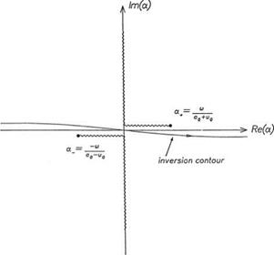
where the left (right) equality sign is to be used when ш is real and positive (negative). The branch cut configuration and the position of the inverse a-contour are shown in Figure 5.3. This configuration is valid regardless whether ш is real and positive or negative. In the в plane the integrand of Eq. (5.18) has a simple pole at в± in the upper half-plane and a simple pole at в_ in the lower half-plane (see Figure 5.4). For y > 0 (y < 0), the inversion contour may be closed in the upper (lower) half­plane by adding a large semicircle as shown (by Jordan’s lemma). By invoking the

Figure 5.3. The branch cut configuration and inversion contour in the complex a plane.

Residue Theorem, the expressions for p and p simplify to

(5.22)

In Eq. (5.22), r and в are the polar coordinates and Ф = a cose + i[a2 – (m – aw0)2/a2 ]1/2 sine.

In the far field, where r ^ to, the а-integral of Eq. (5.22) can be evaluated by the method of stationary phase (see Appendix B). A straightforward application of this method gives

2n

r |Ф"|

Figure 5.4. The poles and inversion con­tour in the complex в plane.

where as is the stationary phase point, вs = в+(as), Ф" (as) = й2Ф/йа2а=а, and V^) = nocos0 + a0(1 – u0 sin20/fl2)i/2. Eq. (5.23) may be rewritten in the more convenient form:

Similarly, the integrals for u and v can be evaluated. The complete asymptotic solution has the following form:

where

V(в) = u0cosв + a0(1 – M2sin2 в)2; M = u0/a0

„ cos в – M(1 – M2sin2 в)1/2 u^’) (1 – M2sin2 в)1/2 – M cos в

v(0) = sin в[(1 – M2sin2 в)2 + Mcos в].

V(0) is the effective velocity of propagation in the в – direction. This asymptotic solution and that of the entropy and vorticity waves will become useful later.

5.1 Dispersion Relations and Asymptotic Solutions of the Linearized Euler Equations

Consider small-amplitude disturbances superimposed on a uniform mean flow of density p0, pressure p0, and velocity u0 in the x direction (see Figure 5.1). The linearized Euler equations for two-dimensional disturbances are as follows:

d U 9 E 9 F

dt dx dy

where

The nonhomogeneous term H on the right side of Eq. (5.1) represents distributed time-dependent sources.

The Fourier-Laplace transform f (а, в, *) of a function f(x, y, t) is related to the function by

to to

f(a, e,v) = II I f (x, y, t)e-i(ax+ey-*)dxdydt

0 —to

TO

f (xy-‘) = f(a-f>-^e’-"da de d*

Г —to

In these equations, the contour Г is a line parallel to the real axis in the complex * plane above all poles and singularities of the integrand (see Appendix A).

Now, consider the general initial value problem governed by the linearized Euler equation (5.1). The initial condition at t = 0 is

u = “initial (x, y)- (5.2)

Figure 5.1. Sources of acoustic, vortic – ity, and entropy waves in a uniform flow.

The general initial value problem for arbitrary nonhomogeneous source term H can be solved formally by Fourier-Laplace transforms. As shown in Appendix A, the Laplace transform of a time derivative is

The Fourier-Laplace transform of Eq. (5.1) is a system of linear algebraic equations that may be written in the following form:

AU — G,

where

and i[H )] represents the sum of the transforms of the source term

and the initial condition.

It is easy to show that the eigenvalues X and eigenvectors Xj (j — 1, 2, 3, 4) of matrix A are

X1 — X2 — (o au0)

X3 — (o — aU0) + $0 (a + в ) X4 — (o — au0) — a0 (a2 + в2)

where a0 = (yp0/p0)1/2 is the speed of sound. The solution of Eq. (5.4) may be expressed as a linear combination of the eigenvectors as follows:

The coefficient vector C, having elements Cj (j = 1 to 4), is given by

C = X-1G. (5.10)

X 1 is the inverse of the fundamental matrix:

Eq. (5.9) represents the decomposition of the solution into the entropy wave, X1, the vorticity wave, X2, and the two modes of acoustic waves, X3 and X4. Now, each wave solution will be considered individually.

5.1.1 The Entropy Wave

The entropy wave consists of density fluctuations alone; i. e., u = v = p = 0. By inverting the Fourier-Laplace transform, it is straightforward to find that p is given by

TO

p(x, y, t) = [ [ [ ———– C—— e'(ax+ey—ot’ida de dox (5.12)

J J J (o – au0)

Г —то

The zero of the denominator gives rise to a pole of the integrand. The relationship between o, a, and в arising from this zero is the dispersion relation. In this case, it is

X1 = (o — au0) = 0. (5.13)

C1 may have poles in the o plane. This is due to periodic forcing. If the wave is excited by initial condition alone, then C1 is independent of o.

In the a plane, the zero of the integrand of Eq. (5.13) is given by

a = — (Im (o) > 0 when o is on Г).

u0

The a-integral of Eq. (5.12) may now be evaluated by means of the Residue Theorem. For x > 0, Jordan’s Lemma requires the completion of the contour on the top half

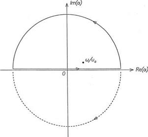Figure 5.2. Inversion contours and pole in the complex a plane.

a plane as shown in Figure 5.2. For x < 0, the contour is completed in the lower half-plane. Thus,

5.1.2 The Vorticity Wave

The vorticity wave consists of velocity fluctuations alone. That is, there are no

The integral in Eq. (5.16) may be evaluated in the same way as that in Eq. (5.12). This leads to

x(x – u0t, y) x ^ TO 0, x ^ —to

Just as for entropy waves, the vorticity wave is convected downstream as a frozen pattern at the speed of the mean flow.