Our heavyweight helicopter equal in the world does not have
In Rostov started production of the most load-lifting rotary-wing car The Russian holding «Helicopt[...]

Everything about aircrafts and helicopters. News and events in aviation worldwide. Civil, transportation, military helicopters and airplanes.

Everything about aircrafts and helicopters. News and events in aviation worldwide. Civil, transportation, military helicopters and airplanes.

Everything about aircrafts and helicopters. News and events in aviation worldwide. Civil, transportation, military helicopters and airplanes.

Everything about aircrafts and helicopters. News and events in aviation worldwide. Civil, transportation, military helicopters and airplanes.


The ghost point method has been extended to treat curved walls in two dimensions by Kurbatskii and Tam (1997). In general, depending on the geometry of the boundary curve and the Cartesian mesh, ghost points can be classified into many types. One major difference between the ghost values associated with curved walls and those of a straight wall aligned with a mesh line is that the ghost values are coupled together. They form a linear matrix system that has to be solved at the end of each time step. Another difference is that there is a stronger tendency for a curved wall to generate high wave number (grid-to-grid oscillations) spurious numerical waves. To ensure stability, a large amount of artificial selective damping is necessary (artificial
|
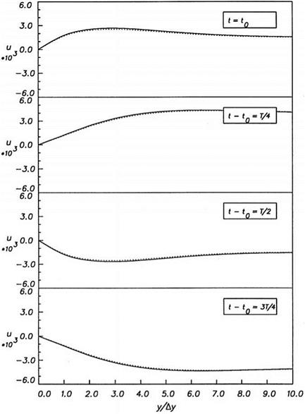
Figure 6.16. Velocity profile of an oscillatory viscous boundary layer at each quarter cycle. Full line is the numerical solution. Dotted line is the Stokes solution. |
selective damping will be discussed Chapter 7). This tends to degrade slightly the quality of the computed solution. A detailed discussion of the method is beyond the scope of this book. Interested persons should consult the original work.
To demonstrate the effectiveness of the proposed numerical viscous boundary conditions for a solid wall, the case of an oscillating viscous boundary layer is simulated. The oscillating boundary layer is generated by a time periodic source in the energy equation at a very low frequency. Upon writing out in full, the energy equation, including the source term, is as follows:
![]()
![]() d p д u д V
d p д u д V
— +——– 1— = 0.01 exp
dt дх д y F
All the viscous stress terms of Eq. (6.16) are included in the computation. To ensure that there are at least 7 to 8 mesh points in the boundary layer (so that it can be resolved computationally) the mesh Reynolds number, R = р0а0Ах//л is taken to be 5.0, and the oscillation period set equal to 1250 time steps (at At = 0.07677). An exact solution of this problem is not available. However, far from the source, the boundary layer resembles the well-known Stokes oscillatory boundary layer. In the Stokes boundary layer the oscillatory velocity component u is given by the following formula:
In Eq. (6.25), the amplitude and phase factors є and 5 are constants of the Stokes solution. For the purpose of comparison with numerical solution, these two constants are determined by fitting solution (6.25) to the numerical solution at the point of maximum velocity fluctuation at two instants of time.
Figure 6.16 shows the computed velocity profile of the oscillating boundary layer along the wall at x = 0. In this figure, T is the period of oscillation. Shown also are the velocity profile of Eq. (6.25) at every quarter period. The agreement between the results of the numerical simulation and the approximate analytical solution appears to be good. On considering that only 7 to 8 mesh points are used to resolve the entire viscous boundary layer, the performance of the numerical viscous boundary conditions and the DRP scheme must be regarded as very good.
To test the efficacy of the inviscid solid wall boundary condition in the presence of a mean flow, this acoustic pulse problem is modified to include a uniform stream of Mach number 0.5 flowing parallel to the wall. In this case, the reflection process is modified by the effect of mean flow convection. For this problem, a computational domain -100 < x < 100, 0 < y < 200 is used. The wall is at y = 0. The linearized Euler equation in two dimensions is as follows:
|
p |
Mp + u |
v |
|||
|
d |
u |
d + dx |
Mu + p |
d + 9 y |
0 |
|
dt |
v |
Mv |
P |
||
|
p |
Mp + u |
v |
|
= 0, |
where M = 0.5. The initial conditions are
t = 0, u = v = 0
The exact solution of this problem is available. Let
a = (ln2)/25, n = [(x – Mt)2 + (y – 25)2]2, g = [(x – Mt)2 + (y + 25)2]1.
|
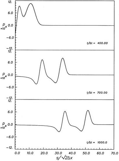
Figure 6.14. Pressure waveforms of an acoustic pulse reflected off a solid wall along the line x = y. |
The solution is
TO TO
и = 0.01 ^ 2qM^ / e 4a sin^^г )J1 df + 0-01 ^ e- 4“ sin(^tJ (f^)f df
0 0
TO TO
(y — 25) f2 (y — 25) f2
v = 0-01 yon – e— 4a sin(ft)J1 (fn)f df + 0.01 y^ e— 4a sin(ft J(fg)f df
00
TO
0-01 f2
p = P = ~2a e 4a cos(ft)[J0(fn) + J0(fs0]fdf,
0
where J0(z), J1 (z) are Bessel functions of order 0 and 1.
|
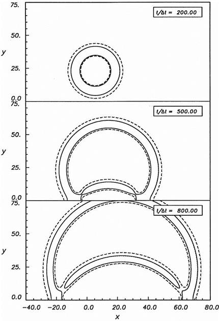
Figure 6.15. Pressure contour patterns associated with the reflection of an acoustic pulse by a solid wall in the presence of a Mach 0.5 uniform mean flow. |
Figure 6.15 shows the computed pressure contour patterns of the acoustic pulse, with the use of the 7-point DRP scheme, at 200, 500, and 800 time steps. Again, the computed pressure contours are indistinguishable from those of the exact solution. Geometrically, the pressure contour patterns are identical to those without mean flow (see Figure 6.13). The uniform mean flow translates the entire pulse downstream at a Mach number of 0.5. The good agreement between the computed and the exact
solutions suggests that the ghost point numerical boundary conditions can be relied upon to simulate correctly a solid boundary even in the presence of a flow.
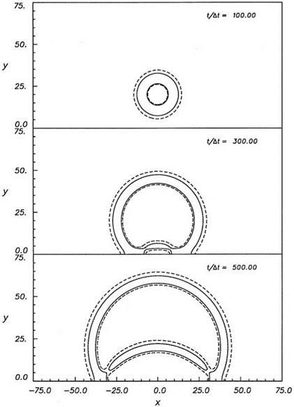
Consider the reflection of a two-dimensional acoustic pulse by a plane wall as shown in Figure 6.13. The fluid is inviscid and is at rest at time t = 0. An acoustic pulse is generated by an initial pressure disturbance with a Gaussian spatial distribution centered at (0, 20). The wall is located at y = 0. The initial conditions are as follows:
![]() – ln 2[x2 + (y – 20)2]
– ln 2[x2 + (y – 20)2]
![]() u = v = 0.
u = v = 0.
In the numerical simulation, the 7-point DRP scheme is used, and the time step At is set equal to 0.07677. This value of At satisfies numerical stability requirement and ensures that the amount of numerical damping due to time discretization is insignificant.
Figure 6.13 shows the calculated pressure contour patterns associated with the acoustic pulse at 100, 300, and 500 time steps. The corresponding contours of the exact solution are also plotted in this figure. To the accuracy given by the thickness of the contour lines, the two sets of contours are almost indistinguishable. At 100 time steps, the pulse has not reached the wall, so the pressure contours are circular. At 300 time steps, the front part of the pulse reaches the wall. It is immediately reflected back. At 500 time steps, the entire pulse has effectively been reflected off the wall, creating a double-pulse pattern: one from the original source, and the other from the image source below the wall.
Figure 6.14 shows the computed pressure waveforms along the line x = y. The distance measured along this line from the origin is denoted by s. The computed waveforms at 400, 700, and 1000 time steps are shown together with the exact solution. As can be seen, there is excellent agreement between the exact and computed results. At 400 time steps, the pulse has just been reflected off the wall. At 700 time steps, the double-pulse characteristic waveform is fully formed. Both pulses propagate away from the wall with essentially the same waveform. The amplitude, however, decreases at a rate inversely proportional to the square root of the distance.
To assess the effectiveness of the ghost point solid wall boundary conditions, a number of direct numerical simulations have been carried out. Comparisons between numerical and analytical solutions are made. This permits an evaluation of the fidelity of both the proposed inviscid and the viscous boundary conditions. In all the examples discussed below, dimensionless variables are used. The characteristic scales are as follows:
length scale = Ax = Ay (mesh size) velocity scale = a0 (speed of sound) Ax
time scale = —
a0
density scale = p0 (ambient density) pressure scale = p0a0
|
A detailed analytical analysis of the reflection of acoustic waves from a wall (see Figure 6.8) using the solid wall boundary conditions described above has been carried out by Tam and Dong (1994). Their analysis clearly shows that, in addition to the reflected acoustic wave, spurious waves (parasite waves) are reflected off the wall. Furthermore, spatially damped numerical waves of the computation scheme are also excited at the wall boundary. These waves form a numerical boundary layer. Space limitations would not allow a discussion of the analytical part of their work. However, their numerical results are useful to provide an assessment of the accuracy and quality of solution in adopting the ghost point method to enforce wall boundary conditions.
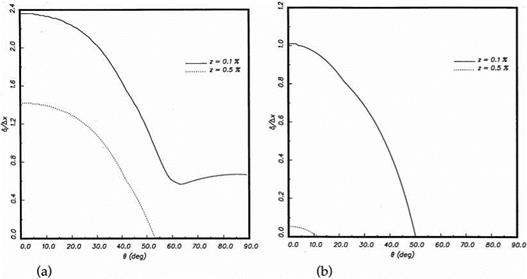
Suppose numerical boundary layer thickness, 8z, is defined to be the distance between the wall and where the spurious numerical wave solution drops to z times the magnitude of the reflected acoustic wave amplitude, e. g., 50 005 denotes the boundary
|
Figure 6.9. Thickness of numerical boundary layer. (a) X/Ax = 6, (b) X/Ax = 10. |
layer thickness based on 0.5 percent of the reflected wave amplitude. Figure 6.9a shows the calculated numerical boundary layer thickness as a function of the angle of incidence when a spatial resolution of X/Ax = 6 (Ay = Ax) is used for computing the acoustic waves; X is the wavelength. Two thicknesses are shown, one corresponds to z = 0.005 (0.5 percent), the other z = 0.001 (0.1 percent). This figure indicates that the numerical boundary layer is thickest for normal incidence. In this case 50 001 is almost equal to 2.5 Ax. Figure 6.9b shows the corresponding numerical boundary layer thickness if a spatial resolution of X/Ax = 10 is used in the computation. It is clear that with better spatial resolution the numerical boundary layer thickness decreases.
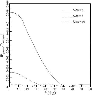
Figure 6.10 shows the dependence of the magnitude of the reflected parasite wave (grid-to-grid oscillations), |pparasite/PincidentI, on the angle of incidence for different spatial resolution. At X/Ax = 6, the reflected parasite wave can be as large as more than 1 percent of the incident wave amplitude at normal incidence. At glazing incidence, i. e., beyond в = 50°, there is generally very little parasite wave reflected off the wall. The magnitude of the reflected parasite wave would be greatly reduced if the spatial resolution in the computation is increased. By using 10 or more mesh points per acoustic wavelength in the computation, the reflected parasite wave is so weak that they may be ignored entirely.
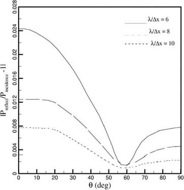
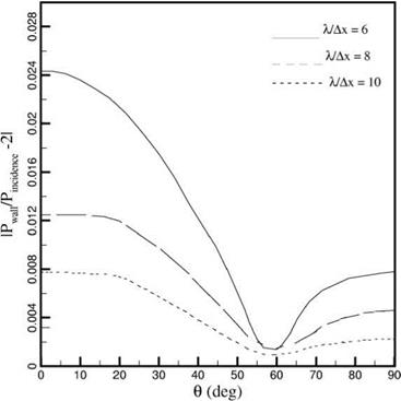
Figure 6.11 is a plot of the deviation from perfect acoustic reflection. It is a measure of the quality of the numerical solid wall boundary condition. For perfect reflection, the ratio of the reflected wave amplitude to that of the incident wave, IPreflected/PincidentI, is unity. Figure 6.11 shows that, by using the proposed numerical solid wall boundary condition, the deviation from perfect reflection is small. It is of the order of 1 percent even when only 6 mesh points per acoustic wavelength are used in the computation. When acoustic waves impinge on a wall, the pressure at the wall is twice the incident sound pressure. This phenomenon is usually referred to as pressure doubling. Figure 6.12 shows that the computed wall pressure would,
|
Figure 6.10. Magnitude of reflected parasite waves as a function of в. |
|
Figure 6.11. Magnitude of reflected wave. |
|
Figure 6.12. Dependence of wall pressure on в. |
indeed, be close to twice the incident sound pressure level for X/Ax = 6. Again, when a better spatial resolution is used in the computation, e. g., X/Ax = 8, the computed results would better reproduce the pressure-doubling phenomenon.
 |
Consider two-dimensional small-amplitude disturbances superimposed on a uniform mean flow of density p0, pressure p0, and velocity u0 in the x direction. The linearized Navier-Stokes equations may be written in the following form:
(T )(n) = (T )(n) = „ Lи») + _!_v
![]()
![]()
 |
(Txy )l, m = (Tyx )l, m = r uj д yul, m+j + д%у j=-3 z y
where l, m are the indices of the mesh points and the superscript n is the time level. If U = Uinitial at t = 0 is the initial condition for the Navier-Stokes or Euler equations, the appropriate initial conditions for the DRP scheme (6.19) are
U(0m = Uinitial’ UUn = 0 fornegative П. (6.20)
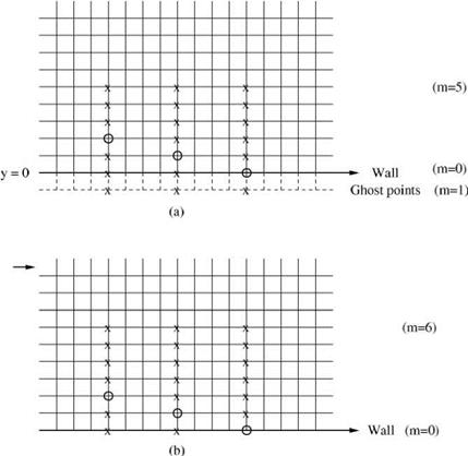
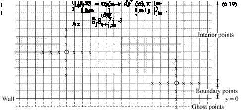
Suppose the fluid is inviscid and a solid wall lies at y = 0 as shown in Figure 6.6. For points lying three rows or more away from the wall, the computation stencil for them lies entirely inside the physical domain. They are referred to as interior points. For the first three rows of points adjacent to the wall, their 7-point stencil will extend outside the physical domain. They are referred to as boundary points. The points outside the computation domain have no physical meaning. They are called ghost points.
Although ghost points are fictitious points with no physical meaning, they are necessary for high-order finite difference schemes. To see this, recall that the solution of the Euler or Navier-Stokes equations satisfies the partial differential equations at every interior or boundary point. In addition, at a point on the wall, the solution also satisfies the appropriate boundary conditions. Now, the discretized governing equations are no more than a set of algebraic equations. In the discretized system, each flow variable at either an interior or boundary point is governed by an algebraic
equation (a discretized form of the partial differential equations). The number of unknowns is exactly equal to the number of equations. Thus, there will be too many equations and not enough unknowns if it is insisted that the boundary conditions at the wall are satisfied also. This is, perhaps, one of the major differences between partial differential equations and finite difference equations. However, the extra conditions imposed on the flow variables by the wall boundary conditions can be satisfied if ghost values are introduced. The number of ghost values is arbitrary, but the minimum number must be equal to the number of boundary conditions. For an inviscid flow, the condition of no flux through the wall requires a minimum of one ghost value per boundary point on the wall. For two-dimensional viscous flow, the no-slip boundary condition requires a minimum of two ghost values per boundary point on the wall for two-dimensional problems. In principle, one can introduce more than the minimum number of ghost values. But for each extra ghost value, a condition must be imposed so that it can be uniquely determined. Clearly, the quality of the solid wall boundary conditions in terms of acoustic wave reflection, acoustic boundary layer characteristics, etc., would be affected by these extra ghost values. Since there is no compelling advantage to introduce extra wall boundary conditions, in the present approach, only the minimum number of ghost values is used.
To fix ideas, let us first consider an inviscid fluid adjacent to a solid wall at y = 0 (see Figure 6.6). In this case, the wall boundary condition is v = 0at y = 0, where (u, v) are the velocity components in the x and y direction, respectively. Since there is one boundary condition, one ghost value is needed for each boundary point at the wall. Physically, the wall exerts a pressure on the fluid with a magnitude just enough to make v = 0 at its surface. This suggests that a ghost value inp (pressure) at the ghost point immediately below the wall should be used to simulate the pressure exerted by the wall. Because only one ghost value is adopted, the difference stencil for the y derivative in the boundary region needs to be modified. Here, it is proposed that the y derivatives are to be computed according to the backward difference stencils shown in Figure 6.7. According to this scheme, the quantities dp/dy, du/dy, and dv/dy are all calculated using values of the variables lying inside the physical domain. For the y derivative of p the stencils extend to the ghost point below the wall. Now, the ghost value of p at the ghost point (l, -1) or pf-1 is to be chosen so that vfl is zero for all n. This can be accomplished through the discretized form of the y-momentum equation (the third equation of Eq. (6.16)), which is used to calculate the value of v at the next time level). Upon incorporating the backward difference stencils of Figure 6.7, the y-momentum equation at a wall point (l, 0) is
3
where a51 are the optimized coefficients of the backward difference stencil. Equations (6.21) and (6.22) are to be used to find vf^1 after all the physical quantities except pne -1, the ghost value, are found at the end of the nth time level computation. To ensure that the wall boundary condition vl"0+1) = 0 is satisfied, the ghost value pf-1
|
may be found by setting v("+1) = 0 in Eqs. (6.21) and (6.22) and then solve for pf-1 This gives
5
Eq. (6.23) is tantamount to setting the ghost value such that 9p/дy = 0 at the wall. It is worthwhile to point out that if no ghost value is introduced, and the boundary condition vf0 is imposed, Eq. (6.21) or its equivalent will, in general, not be satisfied. This means that дp/дy of the solution so computed would not necessarily be equal to zero at the wall.
Now attention is turned to a viscous compressible fluid. In this case, the viscous stress terms of Eqs. (6.16) and (6.17) are to be retained. The stresses are physical quantities and can be computed from the velocity field by the same 7-point difference stencil at an interior point or by the backward difference stencils of Figure 6.7 at a boundary point. For example, at an interior point (1, m), the shear stress тxy at the nth time level is given by
Figure 6.8. Plane acoustic waves incident on a wall at an angle of incidence of в.
where д is the shear viscosity coefficient. (Note: The stress terms are calculated and stored at each time level as a part of the solution. The derivatives of the stresses are computed by the first derivative stencil applied directly on the stresses. No second derivatives need be computed.) At the wall, the no-slip boundary condition u = v = 0 must be enforced. Two ghost values are, therefore, needed per each boundary point at the wall. On following the inviscid case, the ghost value pf-_1 will again be used to ensure that v(n0 = 0 for all n. Physically, in addition to applying a pressure on the fluid normal to the wall, the wall also exerts a shear stress т xy on the fluid to reduce the velocity component u to zero at its surface. This suggests that a ghost value (тху )f-_1 be included in the computation. To enforce boundary condition u(n0 = 0, it is noted that u is determined by advancing the x-momentum equation in time. By following the treatment of v = 0, it is recommended that the у derivative of тxy in the x-momentum equation be approximated by the same backward finite difference stencils as those for p (see Figure 6.7). It is easy to see that the ghost value (тху )(n 1 can be found (in exactly the same way by which the ghost value p(en)_1 is determined) by imposing the no-slip boundary condition u(n0+1) = 0 on the x-momentum equation at the boundary point (l, 0) at the wall. In this way, a unique solution satisfying both the discretized form of the Navier-Stokes equations and the no-slip boundary conditions can be calculated.
Large-stencil finite difference methods are used for CAA problems because they are generally less dispersive and less dissipative, and they tend to be more isotropic. In addition, they yield numerical wave speeds that are nearly equal to the wave speeds of the original partial differential equations. On the other hand, large-stencil or high – order methods support spurious numerical waves. These waves are contaminants or pollutants of the numerical solution. Some of these spurious waves have very short wavelengths (grid-to-grid oscillations) and propagate with ultrafast speeds. They have been referred to as parasite waves. Other spurious waves are spatially damped. Their presence is, therefore, confined locally in space. To ensure a high-quality
computational aeroacoustics solution, it is important that these spurious waves are not excited in the computation.
For inviscid flows, the well-known boundary condition at a solid wall is that the velocity component normal to the wall is zero. This condition is sufficient for the determination of a unique solution to the Euler equations. When a large-stencil finite difference scheme is used, the order of the difference equations is higher than that of the Euler equations. Thus, the zero normal velocity boundary condition is insufficient to define a unique solution. Extraneous conditions must be imposed. Unfortunately, these extraneous conditions would often lead to the generation of spurious numerical waves as mentioned before. The net result is the degradation of the quality of the numerical solution. The degradation may be divided into three types. First, if an acoustic wave is incident on a solid wall, perfect reflection (e. g., reflected wave amplitude equal to incident wave amplitude) may not be obtained. Second, parasite waves may be reflected off the solid surface. Third, a numerical boundary layer can form adjacent to the solid wall surface by the spatially damped spurious numerical waves.
Radiation boundary condition (6.2) and outflow boundary condition (6.13) were derived for a uniform mean flow in the x direction. In many problems, the mean
flow is not in the x direction. However, if the mean flow is not in the x direction, and even has slow spatial variation, Eqs. (6.2) and (6.13) may be extended to account for a general direction and for a slightly nonuniform mean flow. Let the nonuniform mean flow in the boundary region of the computation domain be (p, u, v, p), then a generalization of radiation boundary condition (6.2) (see Tam and Dong, 1996) is
![]() (6.14)
(6.14)
where V (r, d) = u cos в + v sin в + [a2 – (v cos в – u sin в)2]1/2 and a is the local speed of sound. Note: The variables in Eq. (6.2) are the perturbation quantities, whereas (p, u, v, p) are the full variables.
The generalized outflow boundary conditions are as follows:
d u _ 1 d _
— + v ■ v (u – u) = — — (p – p)
dt p dx
9 v _ 1 9 _
— + v ■ V (v – v) = –— (p – p)
91 p dy
where v = (u, v).
It is worthwhile to point out that radiation boundary condition (6.14) allows an automatic adjustment of the mean flow. For time-independent solution, this equation has a solution in the following form:
_ A
(v – v) = Г1/2 ’
and similarly for the other variables. Thus, this set of boundary conditions permits a steady entrainment of ambient fluid when the computed solution requires.
To show the effectiveness of the DRP schemes and the radiation and outflow boundary conditions, the results of one special initial value problem involving all three types of disturbances will be presented below in some detail. The case under consideration consists of an acoustic pulse generated by an initial Gaussian pressure distribution at the center of the computational domain as shown in Figure 6.2. The mean flow Mach number is 0.5. Downstream of the pressure pulse, at a distance equal to one-third of the length of the computational domain, a vorticity pulse and an entropy pulse (also with Gaussian distribution) are also generated at the initial time. Since the acoustic pulse travels three times faster than the vorticity and entropy pulses in the downstream direction, this arrangement ensures that all the three pulses reach the outflow boundary simultaneously. In this way, it is possible to obtain a critical test of the effectiveness of the radiation as well as the outflow boundary conditions in a single simulation.
In the simulation, the variables are nondimensionalized by the following
scales:
length scale = Дх = Ду velocity scale = a0
time scale = —
a0
density scale = p0 pressure scale = p0a0.
The computational domain is divided into a 200 x 200 mesh. The initial conditions imposed at time t = 0 are as follows:
p = e1 exp[-a1 (x2 + y2)] 1 (acoustic pulse)
p = e1 exp[-a1 (x2 + y2)] I + e2exp[-a2((x – 67)2 + y2)] (entropy pulse)
![]() u = e3y exp[-a3((x – 67)2 + y2)] v = – e3(x – 67) exp[-a3 ((x – 67)2 + y2)]
u = e3y exp[-a3((x – 67)2 + y2)] v = – e3(x – 67) exp[-a3 ((x – 67)2 + y2)]
where e1 = 0.01, e2 = 0.001, e3 = 0.0004, a1 = (ln2)/9, a2 = a3 = (ln2)/25. The exact solution (see Tam and Webb, 1993) is.
6.4.1 Acoustic Waves
TO
u(x, y, t) = Є^2а Г/ e-^/4a1 sin(H t)J1 (Hn)H dH 10
TO
v(x, y, t) = j e-H2/4“i sin(Ht)J1 (Hn)HdH
10
TO
p(x, y, t) = p = j e-2/4a1 cos(Ht J(Hn)HdH,
10
where n = [(x – Mt)2 + y2]1/2, J1 and J0 are the Bessel functions of order 1 and 0. M is the Mach number.
6.4.2 Entropy Waves
p = u = v = 0, p = e2eTO[(x-61-Mt )2+y2].
6.4.3 Vorticity Waves
p=p=0
u(x, y, t) = e3ye-“3[(x-61-Mt)2+y2]
v(x, y, t) = – e3(x – 61 – Mt)e-аз[(x-61-Mt)2+y2].
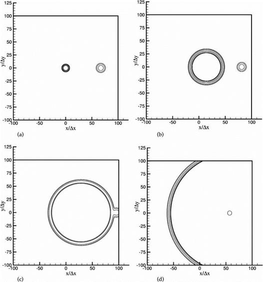
The results of the simulation will now be presented. Figure 6.3a shows the density contours of the acoustic pulse at the center of the computation domain and the entropy pulse downstream at time t = 0. The vorticity pulse has no density fluctuations and, therefore, cannot be seen in this figure. Figure 6.3b shows the computed density contours after 500 time steps (At = 0.0569). At this time, the radius of the acoustic pulse has expanded considerably, while that of the entropy pulse remains the same. The centers of the two pulses have moved downstream by an equal
|
Figure 6.3. Density contours. (a) t = 0, (b) t = 500 At, (c) t = 1000 At, (d) t = 2000 At. |
distance. Figure 6.3c shows the locations of the two pulses at 1000 time steps. The acoustic pulse has now caught up with the entropy pulse. At a slightly later time, the density contours of the two pulses merge and exit the outflow boundary together. Based on the 1 percent contour plot, no noticeable reflections have been observed, indicating that the outflow boundary condition is transparent. At a still later time, the acoustic pulse reaches and leaves the computation domain through the top and bottom boundaries. Again, few or no reflections can be found (to 1 percent of the incident wave amplitude). This is shown in Figure 6.3d. Finally, at 3200 time steps, the acoustic wave front reaches the inflow boundary on the left. The pulse exits the computation domain again with few observable reflections. Contours of the exact
|
|
solution are also plotted in these figures. However, the difference between the exact and numerical solution is so small, they cannot be easily seen.
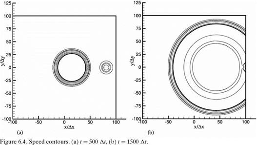
Figure 6.4a shows the contours of the magnitude of the velocity fluctuations (or speed) at 500 time steps. The center circles are those of the acoustic pulse. The circles to the right are contours associated with the vorticity pulse. The contours are constructed by interpolation between mesh points. To the accuracy allowed by this procedure, the expanding circles are, indeed, circular so that the computed acoustic wave speed is the same in all directions. Figure 6.4b gives the speed contours at 1500 time steps. At this time, the main part of the acoustic pulse has already left the outflow boundary. The vorticity pulse, having a slower velocity, has, however, not completely left the right boundary. A small piece of it can still be seen just at the outflow boundary. In this figure, the 1 percent contour exhibits some minor wiggles. A closer examination of the computed data indicates that they are generated by the graphic program and not by the simulation.
The computed density waveform along the x-axis at 500 time steps is given in Figure 6.5a. The exact solution is shown by the dotted line. The exact and computed waveforms are clearly almost identical. Figure 6.5b provides both the computed and the exact waveforms at 1000 time steps when the acoustic pulse has caught up with the entropy pulse. Again, there is good agreement between the two waveforms. Extensive comparisons between the computed density, pressure, and velocity waveforms with the exact solution have been carried out at different directions of propagation up to 4500 time steps when nearly all the disturbances have exited the computation domain. Good agreements are found regardless of the direction of wave propagation. Such good agreements are maintained in time up to the termination of the simulation.
In addition to the simulation just described in detail, several series of simulations using more than one acoustic pulse generated at various locations of the computation
domain have been carried out. Good agreements are again found when compared with the exact solutions of the linearized Euler equations. This is true as long as the predominant part of the wave spectrum has wave numbers a and в, such that a Ax and в Ay are both less than 1.1. Overall, the results of all the simulations strongly suggest that the DRP scheme can be relied on to yield accurate results when used to simulate isotropic, nondispersive, and nondissipative acoustic, vorticity, and entropy waves. Furthermore, the scheme can be expected to reproduce the wave speeds correctly.
It is important to point out that the radiation boundary conditions (6.2) and the outflow boundary conditions (6.13) depend on the angle в. If the boundaries are far from the source, then the exact location of the source is not important. But, if the source is close to a boundary, the effectiveness of these boundary conditions would deteriorate because the direction of wave propagation is in error. An extensive series of tests involving an acoustic source put closer and closer to the boundaries have been carried out. The radiation boundary conditions appear to perform quite well even when the center of the acoustic pulse is 20 mesh points away from the boundary. The reflected wave amplitude is generally less than 2 percent of the incident wave amplitude. The outflow boundary conditions, on the other hand, have been observed to cause a moderate level of reflection; 15 percent for acoustic pulse initiated 20 mesh points away. This is true with or without mean flow. Recalling that the radiation and outflow boundary conditions were developed from the asymptotic solutions, the degradation of the effectiveness of the boundary conditions for sources located close to a boundary should, therefore, be expected.