Category COMPUTATIONAL AEROACOUSTICS

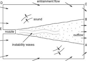
Numerical boundary conditions play a crucial role in the simulation of the jet screech phenomenon. An important requirement of this problem is that the pressure at the nozzle exit and that of the ambient condition are different and must be maintained. It is this pressure difference that leads to the formation of shock cells in the jet plume. Thus, both the outflow and radiation boundary condition must have the capability of imposing a desired ambient pressure to the mean flow solution. For the present problem, several additional types of numerical boundary conditions are required. In Figure 15.53, outflow boundary conditions (see Section 9.3) are imposed along boundary AB. Along boundary BCDE, radiation condition with entrainment flow is implemented (see Section 9.2). On the nozzle wall, the solid wall boundary condition is imposed. The jet flow is supersonic, so the inflow boundary condition can be prescribed at the nozzle exit plane. Finally, the equations of motion in cylindrical coordinates centered on the x-axis have an apparent singularity at the jet axis (r ^ 0). A special treatment, discussed in Section 9.4, is used to avoid the singularity computationally.

All the computations are carried out in the x — r plane. The size of the computational domain is 35D x 17D. By extending the computational domain to 35D downstream, all the screech tone noise sources are effectively included in the computation. Also, the amplitude of the excited instability waves would have decayed significantly at the outflow boundary, thus lessening the likelihood of reflection of unsteady disturbances back into the computational domain. By extending the computational domain to 17D in the radial direction, it is believed that the outer boundary is approximately in the far field. By measuring the radiation angle from the location in the jet where tone emission is the strongest, accurate screech tone directivity can be determined.

The computational domain is divided into four subdomains each having a dif­ferent mesh size as shown in Figure 15.54. The subdomain immediately downstream of the nozzle exit, where the jet mixing layer is thin and the jet plume contains a shock cell structure, has the finest mesh: Ax = Д r = D/64. The mesh size of the next subdomain increases by a factor of 2. This continues on so that, outside the jet where
the mesh is the coarsest, has a mesh size of D/8. The governing equations in cylindri­cal coordinates are discretized by the multi-size-mesh multi-time-step method (see Chapter 12). The use of multiple time steps is crucial to the computational effort. It greatly reduces the run time of the computer code.

For the purpose of illustrating the essential steps and considerations needed to simulate jet screech computationally, only axisymmetric jet screech is considered (see Shen and Tam, 1998). This is to keep the discussion to a reasonable length. For axisymmetric jet screech associated with jets issued from a convergent nozzle, the jet Mach number is restricted to the range of 1.0 to 1.25. Numerical simulation of jet noise generation is not a straightforward undertaking. Tam (1995) had discussed some of the major computational difficulties anticipated in such an effort. First of all, the problem is characterized by very disparate length scales. For instance, the acoustic wavelength of the screech tone is more than 20 times larger than the initial thickness of the jet mixing layer that supports the instability waves. Furthermore, there is also a large disparity between the magnitude of the fluid particle velocity of the radiated sound and the velocity of the jet flow. Typically, they are five to six orders of magnitude different. To be able to compute accurately the instability waves and the radiated sound, a highly accurate CAA algorithm with shock-capturing capability as well as a set of high-quality numerical boundary conditions are required.

15.6.1.1 Computational Model

For an accurate simulation of jet screech generation, it is essential that the feedback loop be modeled and computed correctly. The important elements that form the feedback loop are the shock cell structure, the large-scale instability wave, and the feedback acoustic waves. In the mixing layer of the jet, turbulence is responsible for its spreading. The spreading rate of the jet affects the spatial growth and decay of the instability wave. Thus, turbulence in the jet plays an indirect but still important role in the feedback loop. The length scales of the instability wave, the shock cells,

Figure 15.53. A sketch of the physical domain to be simulated.

as well as the feedback acoustic waves are much longer than that of the fine-scale turbulence in the mixing layer of the jet. Because of this disparity in length scales, no attempt is made here to resolve the fine-scale turbulence computationally. Based on these considerations, an unsteady RANS model is regarded as adequate. To provide the necessary jet spreading induced by turbulence, the к – e turbulence model is adopted. Here, the к — є model simulates the effect of the fine-scale turbulence on the jet mean flow. In the computation described below, the modified к – e model of Thies and Tam (1996), optimized for jet flows, is used.

Figure 15.53 shows the physical domain to be simulated. The following scales are used in the computations; length scale = D (nozzle exit diameter), velocity scale = aTO (ambient sound speed), time scale = D/aTO, density scale = pTO (ambient gas density), pressure scale pTOa^, temperature scale = TTO (ambient gas temperature); scales for к, e, and ut are a^, a3/D, and aTOD, respectively. The dimensionless governing equations in Cartesian tensor notation in conservation form are as follows:

In these equations, y is the ratio of specific heats, и is the molecular kinematic viscosity. k0 = 10—6 and e0 = 10—4 are small positive numbers to prevent division by zero. The model constants are given in Section 15.5.2. The inverse molecular Reynolds number v/(amD) is assigned a value of 1.7 x 10—6 in the computation. Note that, for the range of Mach numbers and jet temperatures considered, the Pope and Sarkar corrections often added to the k – e model are not necessary and are omitted. Here, only cold jets are considered. For this reason, the Tam and Ganesan hot-jet correction is not needed. Outside the jet flow both k and e are zero. On neglecting the molecular viscosity terms, the governing equations become the Euler equations.

Experimentally, it is found that an imperfectly expanded supersonic jet invariably emits strong tones called screech tones. Jet screech is a fairly complex phenomenon involving several modes of oscillations. When a convergent nozzle is used, it is observed experimentally that the screech modes are axisymmetric at low supersonic Mach numbers. There are two axisymmetric modes. They are usually designated as the A1 and A2 modes (see Figure 15.51). At Mach number 1.3 or higher, the jet screech switches to flapping or helical modes. They are designated as the B and C modes. In Figure 15.51 Xs is the wavelength of the screech tone. Mode switching or staging is quite abrupt. The staging Mach number is found to be very sensitive to ambient experimental environment and also sensitive to upstream conditions of the jet flow. Largely because of this sensitivity, it is known that the staging Mach numbers differ slightly from experiment to experiment. Even in the same facility, they tend to differ somewhat when the experiment is repeated at a later time.

It is known, since the early work of Powell (1953), that screech tones are gen­erated by a feedback loop. Recent works show that the feedback loop is driven by the instability waves of the jet flow. In the plume of an imperfectly expanded jet is a quasiperiodic shock cell structure. Figure 15.52 shows schematically the feedback loop. Near the nozzle lip where the jet mixing layer is thin and most receptive to

Figure 15.52. Schematic diagram of the feedback loop of jet screech.

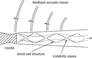external excitation, acoustic disturbances impinging on this area excite the instability waves. The excited instability waves, extracting energy from the mean flow, grow rapidly as they propagate downstream. After propagating a distance of four to five shock cells, the instability wave, having acquired a large enough amplitude, interacts with the quasiperiodic shock cells in the jet plume. The unsteady interaction gen­erates acoustic radiation, part of which propagates upstream outside the jet. Upon reaching the nozzle lip region, they excite the mixing layer of the jet. This leads to the generation of new instability waves. In this way, the feedback loop is closed.

For engineering applications, sometimes it is sufficient to compute the mean velocity profile of a turbulent flow. For this purpose, it has been recognized that the effect of turbulence on the mean flow may be adequately accounted for by including a turbulence-induced stress field. This is the Boussinesq approach. In this approach, the stress field is modeled by relating it to the strain rate field of the mean flow similar to that of laminar flow. This turbulence modeling approach is simple and relatively easy to implement on a computer. For this reason, it has become a wildly popular tool for solving practical problems for which only the mean flow is required.

Turbulence modeling is by now a well-established subject. An in-depth discus­sion of turbulence modeling is beyond the scope of this book. The objective here is to provide an introductory presentation of the subject. There are two most popular two-equation turbulence models. They are the к – є model and the к – ю model (Wilcox, 1998). A one-equation model by Spalart and Allmaras (1994) is also often used. It is now known that the к – є model works well for free shear turbulent flows, while the к – ю model works well for turbulent fluid layers adjacent to a solid surface. Motivated by this observation, Mentor (1994a, 1994b, 1997) has developed combined models, which is a clever way of blending the two models together for

computing boundary layer type flows. In this book, only the к – є model is discussed and only to a limited extent.

The к – є turbulence model has been widely used in association with the RANS equations for turbulent mean flow calculations. However, it has been recognized that the applicability of the original к – є model is quite limited. This is because the model contains only a bare minimum of turbulence physics. Also, it is because the unknown constants of the original model were calibrated primarily by using low Mach number boundary layer and two-dimensional mixing layer flow data [see Hanjalic and Launder (1972), Launder and Spalding (1974), Launder and Reece (1975) and Hanjalic and Launder (1976)].

The useful range of the к – є model has since been extended. The extensions were carried out in two ways. First, a number of correction terms, intended to incor­porate additional turbulence physics in the model, were proposed. Notable model corrections are the Pope (1978) correction developed for use in three-dimensional jets, the Sarkar and Lakshmanan (1991) correction developed for use when the convective Mach number is not too small, and the Tam and Ganesan (2003) correc­tion developed for nonuniform high-temperature flows. Second, for application to a specific class of turbulent flows, the empirical constants of the original model were recalibrated using a large set of more appropriate data. The motivation for recali­bration is the recognition that these constants are not really universal. The model would have a much better chance to be successful if it were applied to a restricted class of flows with similar turbulent mixing characteristics. For each class of flows, a new but more suitable set of constants is used. For instance, for calculating jet and free shear layer mean flows, Thies and Tam (1996) recalibrated the unknown model constants by using a large set of jet flow data covering a wide range of Mach numbers. Their computed jet mean flow velocity profiles for ambient temperature jets were found to be in excellent agreement with experimental measurements. More recently, applications of the recalibrated model to jets in simulated forward flight, coaxial jets, and jets with inverted velocity profile (see Tam, Pastouchenko, and Auriault (2001)) have been carried out with equal success.

The RANS equations including the к – є model in dimensionless form may be written as follows. Here, for jet flows, dimensionless variables with D, Uj, pj, Tj (nozzle exit diameter, jet velocity, density, and temperature) as the length, velocity, density, and temperature scales will be used. Time, pressure, and the turbulence quantities к and є will be nondimensionalized by D/Uj, PjU2j, u2, and uj/D, respec­tively. Turbulent stresses ті;. and eddy viscosity uT will be nondimensionalized by u2 and Uj /D. In Cartesian tensor notation, the Favre-averaged equations of motion including the к – є model, as well as the Pope, Sarkar, and Tam and Ganesan cor­rection terms (in dimensionless form) are as follows:

Continuity

(15.73)

Momentum

dp – d(p Тц)

dxi dxe

where y is the ratio of specific heats, Pr is the Prandtl number, and Mj is the jet Mach number. There are nine empirical constants in the preceding system. The values recommended by Thies and Tam (1996) and Tam and Ganesan (2004) for jet and similar type of flows are as follows:

C, = 0.0874, Ce1 = 1.40, Ce2 = 2.02, Ce3 = 0.822, Cp = 0.035,

YoT = Pr = 0.422, ok = 0.324, ae = 0.377, a = 0.518

The RANS equations and the к – e model were originally developed with the intention for computing the mean velocity profiles of turbulent flows. The question arises as to whether they can be used for computing unsteady flow and noise. For unsteady flow application, the set of equations is, generally, referred to as Unsteady Reynolds Averaged Navier-Stokes (URANS). Clearly, there are limitations to such

usage. However, the system of URANS equations is relatively simple to use. It requires computational resources that are not too demanding. At present, there is no consensus as to whether it is appropriate to use such a formulation for noise prediction. Evidently, for certain types of problems, its use can be justified, whereas for other types it is not. One must decide based largely on the physics of the problem.

It was mentioned at the beginning of this chapter that, at present, there are two approaches to LES. One approach uses a subgrid scale model. The idea is to cut off and not to compute the very high wave number part of the turbulence spectrum. To account for the effect of the cutoff spectrum on the larger-scale turbulent motion, a model of the stress-strain rate relation is used. It turns out that a subgrid scale model based on a stress-strain rate relation does not simulate the effect very well. Such a model effectively provides only damping terms to the fluid motion, especially the high wave number components. This prevents the accumulation of small-scale turbulence energy due to the cascade process (energy continues to cascade to the shorter and shorter scales or higher and higher wave number components). The alternative approach is to use numerical damping to perform the same task. A natural way, in the later case, is to use artificial selective damping. For this purpose, the a = 0.3n damping curve of Section 7.2 may be used. There is no sharp cutoff for this damping curve. A reasonable choice is to take the cutoff wave number to be approximately at a Ax = 1.6.

Instead of using artificial selective damping, one may use filtering. Filtering is a way to eliminate high wave number components with minimal effect on the long waves. A one-dimensional numerical filter may be constructed as follows.

Let f be the value of a dynamical variable at the I th mesh point. Consider a 7-point stencil filter. A filter should be symmetric to avoid any chance of amplifying the filtered value. Suppose f is the filtered value. The filtered value is related to the original values on the computational stencil by the following relation (assuming a linear filter is used).

fl = A( ft+3 + fl-3 ) + B( fl+2 + fl-2) + C( ft+1 + fl-1) + Dfl. (15.66)

The Fourier transform of Eq. (15.66) is

f = [2A cos(3aAx) + 2B cos(2aAx) + 2Ccos(aAx) + D] f = F(aAx) f. (15.67) On inverting the Fourier transform, the filtered function becomes

f(x) = f F(aAx)feiaxda. (15.68)

It is clear that the function F(a Ax) in Eq. (15.68) regulates the band of wave numbers that contributes to the filtered value of the original function. For this reason, F (a Ax) is referred to as the filter function.

1.0

Figure 15.49. An ideal filter with a cutoff : :r v,

at a Ax = pn.

Ideally, if all the wave numbers larger than a Ax > pn associated with a tur­bulence field are to be discarded or ignored, then the desirable filter function would be

This ideal filter function is shown in Figure 15.49. When a finite size stencil is used, it is not possible to construct an ideal filter function. Thus, the objective is to make the filter as close to the ideal filter as possible.

For a 7-point stencil filter function, there are four free parameters. These param­eters will now be determined by requiring the following conditions be satisfied.

F (0) = 1.0

з 2f

d(aAx)2 aAx=0 3 4F

d(aAx)4 aAx=0

F (n) = 0

It is easy to show that the values of the coefficients that satisfy these constraints are as follows:

A = 64^ B = 32’ C = 14- D = 11. (15.70)

Thus the filtering formula is

fl = 64 (ft+3 + fl-3 ) – 32 (ft+2 + fl-2) + 15 (fl+1 + fl-1) + Ц ft. (15.71)

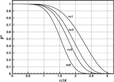
The filter function F (a Ax) is shown as the n = 1 curve in Figure 15.50. This figure does not look like the ideal filter function. To make the filter function resembling more of the ideal filter, one may perform repeated filtering. It is straightforward to show if the filtering process is performed n number of times, the filtered function becomes

TO

f(x) = F (aAx) h. V-da.

— TO

That is, repeated filtering amounts to using a high power of the original filter function. Figure 15.50 shows a plot of F2 (a Ax), F3 (a Ax), F6(a Ax), i. e., n = 2, 3, 6. It is clear that the filter function to a high power has a better resemblance to the ideal filter. However, it is not advisable to perform many filtering operations in one time step, because it will degrade the solution in the long wave range. If n = 3 filter is used, the approximate cutoff wave number, taken to be F3 (acutoff Ax) = 0.5, is given

by acutoffAx ^ 1.8.

In aeroacoustics, turbulence is a principal source of broadband noise. Therefore, research and development of turbulence modeling and turbulence simulation are an integral part of CAA.

Because of the availability of more and more powerful and faster and faster computers, turbulence, nowadays, becomes a favorite activity of large-scale compu­tation. It is known that direct numerical simulation (DNS) of high Reynolds number turbulent flows requires an exceedingly large number of mesh points and long CPU time. On account of such requirements, DNS is presently not considered feasible for solving practical CAA problems. Recently, attention has turned to LES. However, owing to the three-dimensional nature of turbulence, realistically, LES can be car­ried out only in relatively small computational domains. Simple estimates of mesh and computer requirements would convince even the most ardent proponents of LES that it would be sometime in the future, when much more powerful and faster computers become available, before LES would become a design tool in CAA.

The appeal of DNS and LES is that they can, in principle, compute the entire or a large part of the turbulence spectrum. But, for noise prediction, it is highly plausible that it is not necessary to know everything about turbulence or the entire turbulence spectrum. How much does one really need to know about turbulence before one can calculate turbulence noise is an open question. It appears that if one’s primary concern is on the dominant part of the noise spectrum, it is very likely that only the resolution of the most energetic part of the turbulence spectrum is necessary.

Calculating the mean flow velocity profile and other mean quantities of turbulent flows is, in general, important for engineering applications. For mean flow calcula­tion, a practical way is to use the RANS equations with a two-equation turbulence model (e. g., the к – є or the к – ы model) or, if desired, a more advanced model.

The question pertinent to CAA is whether models of a similar level of sophistication could be developed for noise calculation. There is no clear answer to this question. It is a matter of intense research at this time.

In Section 15.4.3, it was demonstrated that the energy source responsible for the gen­eration of airfoil tones is near-wake instability. These are antisymmetric instabilities. However, the flow is at a low subsonic Mach number. It is known that low subsonic flow instabilities are, by themselves, not strong or efficient noise radiators. In this section, the results of a study of the space-time data of the numerical simulations are reported. The objective of the study is to identify the tone generation processes. To facilitate this effort, the fluctuating pressure field p’, defined by,

p’ = p – p, (15.65)

where p is the time-averaged pressure is first computed. Positive p’ indicates com­pression. Negative p corresponds to rarefactions of the acoustic disturbances. Of special interest is the contour p’ = 0. Following Tam and Ju (2012) this contour will be used as an indicator of the acoustic wave front. The propagation of this contour from the airfoil wake to the far field is tracked. The creation and spreading of the wave front provides the clues needed for identifying the tone generation processes.

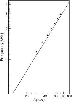
Figure 15.44. Comparison between DNS tone fre­quencies (A) and most amplified instability wave fre­quencies (straight line). Airfoil #1.

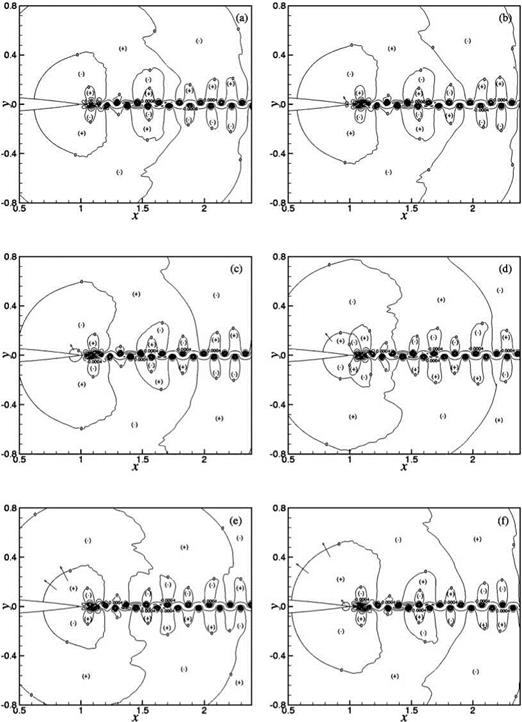
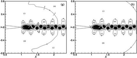
A study of the space-time data reveals that the tone generation processes are rather complex. There is a dominant mechanism involving the interaction between the near-wake oscillations driven by wake instability and the airfoil trailing edge. However, there are also secondary mechanisms arising from flow and vortex adjust­ments in the near wake. Details of these tone generation processes can be understood by following the evolution of the wave front contour p = 0 in time. Figure 15.45 illustrates the dominant tone generation process in space and time. Airfoil #2 (2 percent truncation) at Re = 4 x 105 is used in this simulation. Figure 15.45a may be regarded as the beginning of a tone generation cycle. The trailing edge of the airfoil is shown on the left center of the figure. The flow is from left to right. Thus, the wake, defined by two p’ = 0 contours, lies to the right of the airfoil. The near wake is highly unstable. The instability causes the wake to oscillate as can easily be seen in this figure. The wake is flanked by two rows of vortices in a staggered pattern. The spinning motion of the vortices creates a low-pressure region inside the vortices. Hence, all the vortices are located in the p < 0 regions. These regions are labeled by a (-) symbol. Regions with p > 0 are labeled by a (+) symbol. Shown in Figure 15.45a are wave front contours of p = 0. The near-wake instability is antisymmetric with respect to the x-axis. This leads to an antisymmetric pressure field as shown in Figures 15.45a-15.45h. The pressure field shown in Figure 15.45a corresponds to the beginning of the downward motion of the wake in the region just downstream of the airfoil trailing edge. Since the airfoil is stationary, the downward movement of the near wake leads to the creation of a high-pressure region on the top side of the airfoil trailing edge and a corresponding low-pressure region on the mirror image bottom side. This is shown as two small circular regions right at the trailing edge of the airfoil in Figure 15.45b. A small arrow is inserted there to indicate the direction

of motion of the wave front. The high – and low-pressure regions grow rapidly in time as shown in Figures 15.45c-15.45e. The time difference between Figure 15.45a and Figure 15.45e is nearly half a cycle. Hence, Figure 15.45e to Figure 15.45h repeats a similar sequence of wave front motion, but with positive and negative fluctuating pressure fields interchanged. Each wave front contour in each half-cycle shows its creation at the trailing edge of the airfoil, its expansion in space and time, and its propagation to the far field in all directions.

The dominant tone generation process is observed in all the simulations that have been carried out. In some cases, other less dominant tone generation processes have been observed. These secondary processes may reinforce the primary process or may be important only in certain directions of radiation. By and large, the secondary mechanisms are related to the adjustment of the flow from boundary layer type to free shear wake flow and also the alignment of the wake vortices from their creation to that of a vortex street.

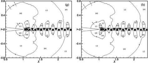
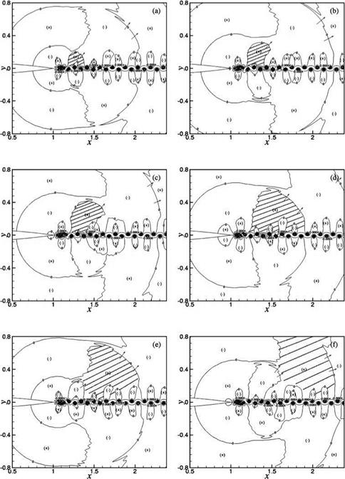
Figure 15.46 illustrates a secondary tone generation process. Figure 15.46a may be taken as the distribution of the wave front contours at the beginning of a cycle for Airfoil #2 at Reynolds number = 2 x 105. At the instant corresponding to Figure 15.46a, the near wake begins to move upward. This creates a high-pressure region on the bottom side of the airfoil trailing edge and, at the same time, a low-pressure region on the mirror image location on the top side. This is shown in Figure 15.46b. Figure 15.46c shows the expansion of the high (bottom)- and low (top)-pressure regions near the trailing edge. At the same time, this figure also shows the expansion of the next two loops; negative-pressure regions on the top half of the figure and positive-pressure regions in the lower half. The three negative-pressure regions that have expanded are labeled as 1, 2, and 3 in this figure. The locations of loops 2 and 3 coincide with the region where the wake oscillations are strongest with largest lateral displacements (see Figure 15.31). However, the wake has not rolled up to form vortices yet. Thus, this secondary tone generation process does not involve the formation of discrete vortices. Figures 15.46d-15.46g show the merging of the loops and the propagation of the wave front to the far field. Therefore, for this case, the adjustment of the near-wake flow assists and contributes to the generation of the observed airfoil tone.

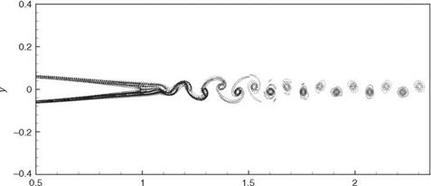
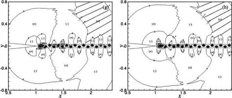
For airfoils with a sharp trailing edge, especially when operating at the high end of the moderate Reynolds number range, the wake rolls up into discrete vortices very close to the trailing edge (see Figure 15.47). In these cases, the formation of discrete vortices does contribute to the generation of airfoil tones. This secondary tone generation process is illustrated in the motion of the wave fronts in Figure 15.48. Figure 15.48a may be considered as the beginning of a tone generation cycle. To observe the secondary tone generation process, attention is directed to the shaded area of this figure. Figure 15.48b (at a later time) shows the expansion of the shaded region. In comparison with Figure 15.47, it is seen that the location of the expanded shaded region coincides with the beginning of the wake rolling up into isolated vortices. It is believed, therefore, that the formation of the vortices is what drives the expansion of the shaded region. Figures 15.48c-15.48h track the continued spreading of the sound pulse after it is generated. It appears that the dominant tone generation mechanism due to the interaction of near-wake instability and the airfoil trailing edge is responsible for the radiating sound to the upstream and sideline directions.

The secondary tone generation mechanism due to the formation of discrete vortices is responsible for radiating sound to the downstream direction. The two mechanisms are perfectly coordinated and synchronized.

A number of investigators, e. g., Tam (1974), Fink (1975), Arbey and Bataille (1983), Lowson et al. (1994), Nash et al. (1999), Desquesnes et al, (2007), Sandberg et al. (2007), Chong and Joseph (2009), and Kingan and Pearse (2009), have suggested that airfoil tones are driven by the instabilities of the boundary layer. Various computa­tions of Tollmien-Schlichting-type instabilities have been performed. The objective is to show that the frequency of the airfoil tone is the same as that of the most ampli­fied instability wave. An examination of the past computation reveals that the spatial growth rate of the Tollmien-Schlichting wave is very small. Only in the separated flow region is there a substantial growth rate. However, all the instability calcula­tions were carried out using the locally parallel flow approximation. Unlike attached boundary layers, the thickness of a separated boundary layer increases rapidly. This makes the appropriateness of the parallel flow approximation questionable. Thus, one should not be too ready to accept the results of past instability calculations without an examination of the approximation adopted in the computation.

In the present study, the NACA0012 airfoil is set at zero degree angle of attack on purpose. At a zero degree angle of attack, there is practically no flow separation on the airfoil until almost the trailing edge. Thus, the spatial growth rate of the Tollmien – Schlichting wave is much smaller than that of the Kelvin-Helmholtz instability in the wake of the airfoil. It is known that the growth rate of Kelvin-Helmholtz instability is inversely proportional to the half-width of the shear layer. In other words, a thin wake is more unstable than a thicker wake. That this is true is shown in Figure 15.40. This figure shows the computed spatial growth rate (antisymmetric mode) over the distance of a chord for Airfoil #1 at different instability wave frequencies. The computations are done using the nonparallel flow instability theory of Saric and

Figure 15.41. Comparison between the spatial growth rates of Kelvin-Helmholtz instability waves at the minimum half­width point using locally parallel (………………………………. )

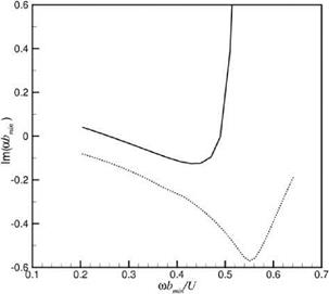and nonparallel (—– ) instability theo­

ries. Airfoil #2, Re = 3 x105.

Nayfeh (1975). The flow in the calculation has a Reynolds number of 3 x 105. The solid curve is for the minimum half-width point of the wake at x/C = 1.088 measured from the leading edge of the airfoil. The dotted curve is for a point in the developed wake region (x/C = 1.556). The maximum growth rate at the thinnest point of the wake is many times larger than that in the developed wake.

By performing instability computation, it is easy to establish that the maximum growth rate occurs in the wake at the location where the wake half-width is minimum. It is believed that because the growth rate is very large, the instability initiated at this region is ultimately responsible for the generation of airfoil tones. The necessary computed instability results to support this hypothesis will now be provided. Because of the rapid growth of the thickness of the wake at the minimum half-width location, Tam and Ju (2012) recognized that the nonparallel flow instability wave theory of Saric and Nayfeh (1975) should be used to perform all instability computations. Their method is a perturbation method. The zeroth order is the locally parallel flow solution. A first-order correction, to account for the spreading of the mean flow, is then computed. The combined growth rate is taken as the nonparallel spatial growth rate. Figure 15.41 shows the difference between parallel and nonparallel spatial growth rates at the minimum wake half-width point for Airfoil #2 at a Reynolds number of 3 x 105. It is straightforward to see from this figure that the nonparallel flow growth rate is smaller. Furthermore, the frequencies of the most amplified wave computed using parallel and nonparallel flow theories are quite different.

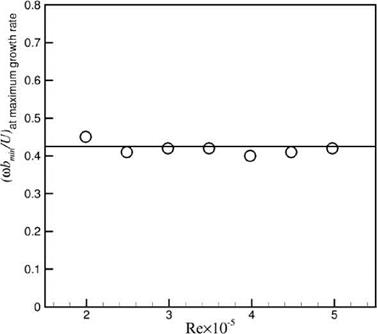
Figure 15.42 shows the angular frequency of the Kelvin-Helmholtz instability wave with the highest amplification rate at the narrowest point of the wake of Airfoil #2 as a function of Reynolds number. When nondimensionalized by minimum half­width bmin and free stream velocity U, the quantity (<& bmin/U) at the maximum growth rate is nearly independent of the Reynolds number. A good fit to the data is as follows”

«4.3. (Airfoil #2). (15.61)

Now, for this airfoil, bmin and Reynolds number are related by Eq. (15.56). By eliminating bmin from Eq. (15.56) and Eq. (15.61), it is found that

0.00835U15 1

(Cu)2

Eq. (15.62) is exactly the same as Eq. (15.59) for Airfoil #2. The K value obtained directly from numerical simulations, displayed in Table 15.3, is in agreement with that from hydrodynamic instability consideration.

A similar nonparallel instability analysis for Airfoil #1 has also been carried out. Figure 15.43 shows the angular frequencies corresponding to that at maximum growth rate nondimensionalized by bmin and U as a function of the Reynolds number. An approximate relationship similar to Eq. (15.61) is

Thus, by eliminating bmin from Eqs. (15.57) and (15.63), a tone frequency formula based on wake instability consideration for this airfoil is

0.00910U15 1

(Cu)2

The proportionality constant in Eq. (15.64) differs slightly from that found from direct numerical simulation as given in Table 5.3. Figure 15.44 shows a direct com­parison between the tone frequencies measured directly from numerical simulations

(triangles) and the most unstable frequencies in the wake at minimum half-width (straight line). The agreement is quite good. It is, therefore, believed that the good agreements for Airfoils #1 and #2 lend support to the validity of the proposition that the energy source of airfoil tones at zero degree angle of attack is near wake flow instability.

In all the simulations that have been performed for Airfoils #1, #2, and #3 (see Table 15.2). only a single tone is detected. Figure 15.37 shows a typical airfoil trailing

edge noise spectrum. This is the noise spectrum of Airfoil #1 at a Reynolds number of 4 x 105. The measurement point is at (1.08, 0.5). Since there is only one single tone per computer simulation, it makes the finding the same as Nash et al. (1999).

Figure 15.38 shows the computed tone frequencies versus flow velocities for Airfoil #1 according to the results of our numerical simulations. This airfoil has a 0.5 percent truncation. It is nearly a sharp trailing edge airfoil. As shown in this figure, all the data points lie practically on a straight line parallel to the Paterson formula (the full line). The difference between the simulation results and the Paterson formula

is very small. On the basis of what is shown in Figure 15.38, it is believed that the simulations, for all intents and purposes, reproduce the empirical Paterson formula. The good agreement with the Paterson formula not only is a proof of the validity of the simulations, but also is an assurance that numerical simulations do contain the essential physics of airfoil tone generation.

Figure 15.39 shows the variations of the Strouhal numbers of the computed tones with Reynolds number for the three airfoils under consideration. The data for each airfoil lies approximately on a straight line. The straight lines are parallel to each

other and to the Paterson formula (shown as the full line in Figure 15.39). All the four lines in Figure 15.39 fit a single formula as follows:

fC 1

Ц – = KRe2, (15.58)

where K is a constant. Eq. (15.58) may also be written in the form similar to the Paterson formula, i. e.,

3

U 2

f = K——– 1. (15.59)

(Cu)2

The values of constant K for each airfoil have been determined by best fit to the simulation data. They are given in Table 15.3.

Based on the computed results shown in Figure 15.39, the effect of trailing edge thickness at a given Reynolds number is to lower the tone frequency, that is, the thicker the blunt trailing edge the lower is the tone frequency. This dependence turns out to be similar to that of vortex shedding tones, such as that emitted by a long circular cylinder in a uniform flow. For the long cylinder vortex shedding problem, the tone Strouhal number is approximately equal to 0.2, i. e.,

fD

— & 0.2 (D is the diameter). (15.60)

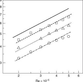Figure 15.39. Dependence of tone Strouhal number on Reynolds number

for Airfoils #1, #2, and #3.—– , Airfoil

#1,…………. Airfoil #2;——– , Airfoil #3;

—– , Paterson formula.

Therefore, the thicker the blunt object or trailing edge, the lower the tone frequency is. However, note that the physics and tone generation mechanisms are quite different.