Category COMPUTATIONAL AEROACOUSTICS

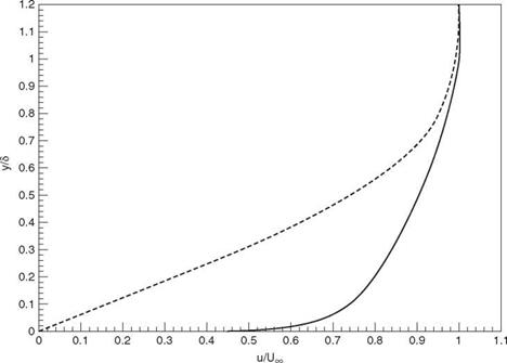
The velocity profile of a turbulent boundary layer over a flat plate consists of three distinct layers. They are the viscous sublayer, the log layer, and the outer wake layer. Figure 15.10 shows the velocity profile of a turbulent boundary layer at low Mach number. The velocity profile is constructed by using the law of the wake profile for the outer layer and Spalding’s formula for the inner layer. The viscous sublayer is very thin and has a very large velocity gradient. It accounts for less than 1 percent of the boundary layer thickness. The log layer lies on top of the viscous layer. It makes up about 20 percent of the boundary layer thickness. The log layer may be regarded as a transition layer. The top layer is the wake flow. It constitutes the bulk (~80 percent) of the boundary layer. In this layer, the velocity gradient is the mildest. Because of the large variation of mean flow velocity gradient across the boundary layer, it is not feasible to use a single size mesh for its computation. The mesh size needed to resolve each of the three layers will be considered separately below.

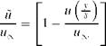
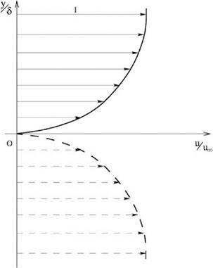
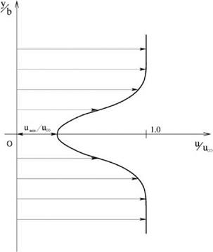
Let the velocity profile of a low-speed flat-plate turbulent boundary layer be u(y/5), where 5 is the boundary layer thickness. As in the case of laminar boundary layer, the velocity deficit U (see Figure 15.11a) may be written in the following form:

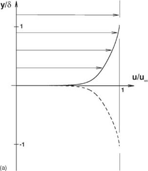Figure 15.11a. Profile of velocity deficit й/и^ of a low-speed turbulent boundary layer.

Figure 15.11b. Profile of velocity deficit u-20%/ure of a low-speed turbulent boundary layer.

The Fourier transform of the velocity deficit, extended to the full range – re < y

< re, is

A change of variable leads to

It is easy to show that the area of the wave number spectrum is unity. Suppose the 7-point stencil DRP scheme is used for computation, then the fractional error в for using a computational mesh size Ay is

°-95( y)

в = 1 — 2 ‘S(Z)dZ. (15.15)

0

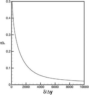
The numerical solution of Eq. (15.15) is given in Figure 15.12. By means of this figure, it is a simple matter to make a quantitative estimate of the maximum mesh size Ay permissible for a prescribed fractional error в. In this way, the mesh size required to compute the viscous sublayer is found.

To find the mesh size needed to resolve the log layer, one may use essentially the same procedure as before. Consider a turbulent boundary layer with the bottom 2 percent removed, that is, the viscous sublayer is taken out from consideration. Let the new mean velocity profile be u—2<% (|). Now, apply this analysis to u -2% (S), the new velocity deficit with a symmetric extension to the negative y plane is

Figure 15.12. Spatial resolution curve for the viscous sublayer of a turbulent bound­ary layer.

The mesh size requirement for computing velocity deficit profile Eq. (15.16) by the 7-point stencil DRP scheme may be determined in the same way as velocity deficit profile Eq. (15.13). Figure 15.13 shows the mesh size resolution curve, в versus 5 /Ay, for computing the log layer of a turbulent boundary layer. This procedure may be applied to the wake layer as well. This is done by deleting the lower 20 percent of the boundary layer velocity profile as shown in Figure 15.11b. On proceeding as

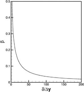Figure 15.13. Spatial resolution curve for the log layer of a turbulent boundary layer.

Figure 15.14. Spatial resolution curve for the wake layer of a turbulent bound­ary layer.

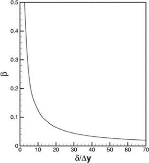above, it is straightforward to derive the mesh resolution curve for computing the outer wake layer. Figure 15.14 is the в versus S/Ay curve.

On comparing Figures 15.12,15.13, and 15.14, it is evident that there are orders of magnitude of difference in the mesh size requirement in computing the three layers of a turbulent boundary layer. This is probably not too surprising. In a realistic computation, a multisize mesh is absolutely necessary. Such a computation can be handled by the multi-size-mesh multi-time-step method discussed in Chapter 12.

Now, boundary layer flows are quite different from free shear layers. Unlike free shear flows, boundary layer flows occupy only a half-infinite space. Furthermore, boundary layers have a substantially different mean velocity profile. Because of these differences, it is necessary to modify slightly the mesh size selection procedure. For example, consider a low-speed flat-plate boundary layer of thickness 5 (99 percent) in a free stream flow of velocity uC. The mean flow has a well-known similarity

Figure 15.8. Velocity profile of a laminar boundary layer and its reflection.

profile. It is given by the Blasius solution (see Figure 15.8). In standard notation (White, 1991), it is as follows:

— = f (n), n = ^ (f (3-5) = 0-99).

йж S

To facilitate the computation of the wave number spectrum, it is recommended to regard the problem as one to compute the velocity deficit as follows:

— (Щ = [1 – f (Ini)] (15.10)

instead of the mean velocity. Note: Eq. (15.10) extends the velocity deficit to the full range —ж < y < ж by a simple reflection.

Now, the Fourier transform of —, denoted by S, is

ж ж

S(ff) = 2П f — (^)e—iaydy = 7- j [1 — f (ini)] Є3-5ndn. (15.11)

— ж —ж

It is easy to show that the area under the wave number spectrum is unity. Therefore, the normalized wave number spectrum is given by Eq. (15.11). Thus, the fractional error by using the 7-point stencil DRP scheme is

0.95

e=1—2 К35)da

Figure 15.6 shows the mean velocity profile of a low-speed two-dimensional turbulent jet. According to White (1991),agood analytical representation of the velocity profile is

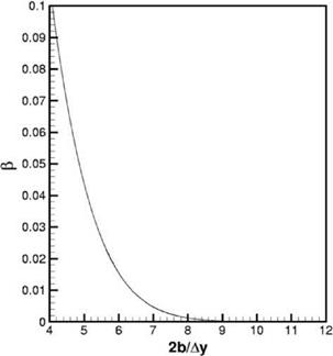
Figure 15.7. Spatial resolution curve for two-dimensional turbulent jets.

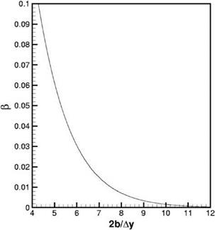
where b is the half-width of the jet. It is easy to show that the Fourier transform of the function on the right side of Eq. (15.3) is

and that

where a = 0.95 /Ay. Figure 15.7 is a plot of в as a function of 2b/Ay. It is the numerical solution of Eq. (15.9). Here again, the 7-point stencil DRP scheme is assumed to be the computational method.

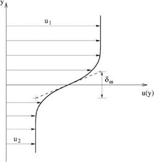
The velocity profile of a low Mach number two-dimensional turbulent mixing layer between two fluid layers of velocities u1 and u2 is shown in Figure 15.4. In nondi­mensional form, the mean velocity profile may be represented analytically (see the book by White) by an error function.

where 8ш is the maximum vorticity thickness defined by

u1 — u2

The velocity profile of a mixing layer tends to a constant as |y| ^ to. For this reason, the profile has no Fourier transform in the usual sense. However, the velocity gradient du/dy is a well-behaved function. It is a well-known fact that the integral of a function is smoother and better behaved than its derivative. Therefore, if the mesh size is chosen to be able to resolve du/dy, then the mesh should be able to provide adequate resolution for computing u(y). Thus, the function to be considered is

Figure 15.5. Spatial resolution curve for two-dimensional mixing layers.

In designing a computational grid, the first question one faces is “what size mesh to use.” This question cannot be answered until one has some idea of the flow and acoustic fields as well as the size of acoustic sources involved. Even if they are known, it is still not straightforward to decide what size mesh to use. For instance, if the flow contains a free shear layer of vorticity thickness, 8a, what mesh size to use is not completely obvious unless one has previous experience. The purpose of this section is to develop quantitative criteria to assist in selecting a proper mesh size for aeroacoustics computation.

15.2.1 Free Shear Flows

As an illustration of how one may formulate a mesh size selection procedure, consider the problem of computing a low Mach number two-dimensional wake flow of half­width b. According to the book by White (1991), the velocity deficit, U, of such a wake flow, whether it is laminar or turbulent, has the profile of a Gaussian function, i. e.,

The velocity profile is shown in Figure 15.1.

For computational purposes, the mesh size is to be assigned so as to be capable of resolving the Gaussian function part of the flow. Now, note that the Fourier transform of a Gaussian function is a Gaussian function, i. e.,

where a is the wave number. It is easy to show that the area under the wave number spectrum of Eq. (15.2) is unity, i. e.,

TO

j S(a)da = 1.

-TO

Figure 15.1. Velocity profile of a two­dimensional turbulent wake.

The fraction of the wave number spectrum up to a wave number k, denoted by F(kb), is

k

F(kb) = 2 j S(a)da = erf
0

where erf [ ] is the error function. If the mesh size is chosen to resolve the wake flow up to a wake number k, then the fractional error, E(kb), is equal to

A plot of E(kb) is shown in Figure 15.2.

Suppose the 7-point stencil DRP scheme is chosen to do the computation. This scheme is acceptable if the mesh size Ay is chosen so that kAy < 0.95 (see Chapter 2). Now consider that a fractional error в (в << 1.0) is acceptable for the computation; then, by using the 7-point stencil DRP scheme, the mesh size would be given by equating E(kb) to в with k = (0.95/Ay). This gives

of 2b/Ay. Now, for an assigned value of в, there is a corresponding value of 2b/Ay, say a. Thus, the maximum mesh size allowed is

2b

(АУ ^maximum = — • (15.6)

a

By following this procedure, the maximum mesh size for a given acceptable error for other shear flows can be readily established. For the cases of a two-dimensional

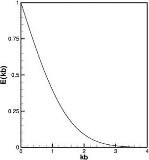Figure 15.3. Spatial resolution curve for two-dimensional wake flow.

Figure 15.4. Velocity profile of a two­dimensional turbulent mixing layer.

mixing layer, a two-dimensional turbulent jet, a laminar boundary layer, and a tur­bulent boundary layer, the spatial resolution curves are provided in the following sections.

Inclusion of artificial selective damping in a computation code is absolutely necessary if a central difference scheme is used. Central difference schemes have no intrinsic damping. Without artificial selective damping, such a computation would fail either because the solution is heavily polluted by spurious waves or through a blowup. In a typical numerical simulation, artificial selective damping has two roles to play. First and foremost, it eliminates spurious waves, especially grid-to-grid oscillations as they propagate across the computation domain. For this purpose, a standard practice is to add a general background damping throughout the entire computation domain. The mesh Reynolds number should be chosen so that any grid-to-grid oscillations are damped by several orders of magnitude when propagating from one side to the other side of a subdomain. The second purpose of imposing artificial selective damping
is to suppress the generation of spurious waves. Spurious waves are produced at surfaces of discontinuities. Thus, at solid surfaces, fluid interfaces, or mesh-size – change interfaces, extra artificial selective damping should be imposed. When a simulation contains solid surfaces with sharp edges and corners, one must recognize that these are sites for the generation of strong grid-to-grid oscillations. Grid-to – grid oscillations are one of the main causes of numerical instability. To suppress the generation of grid-to-grid oscillations, an effective method is to add additional artificial selective damping at and near sharp edges and corners.

What boundary conditions to use in a CAA simulation should be given a good deal of thought. In previous chapters, a variety of numerical boundary conditions was discussed. So, for a given aeroacoustic phenomenon, more than one type of boundary condition may be used. For example, for a radiation boundary, one may use radiation boundary conditions based on asymptotic solution. An equally good, and maybe even better boundary condition, is to use the perfectly matched layer (PML) absorbing boundary condition.

Sometimes, the choice of which numerical boundary condition to use is severely limited, unless some new way to enforce the radiation boundary condition is found. For instance, to compute the noise and flow of an imperfectly expanded supersonic jet, an external boundary condition must be imposed that allows the ambient pres­sure, pa, to be specified. At the nozzle exit, the static pressure of the jet, pexit, is specified by the nozzle flow. Now, the enforcement of the nozzle exit boundary condition p = pexit is relatively straightforward. At the external boundary of the computational domain, the boundary condition must perform two different roles. It must allow the outgoing acoustic waves to exit with little reflection. At the same time, it must require the mean static pressure of the numerical solution to take on the valuepa. Most known absorbing boundary conditions do not have this capability. Among all the boundary conditions discussed in this book, it seems that only the asymptotic radiation boundary condition, discussed in Chapter 6 and Chapter 9, is capable of performing the dual functions.

Although it has been mentioned before, it is worthwhile to reemphasize that the external boundary conditions of a CAA simulation must exert the same influence on the computation as in the physical problem. This includes waves generated outside the computational domain, but propagated into the domain as incident waves. The same is true with mean flow and entrainment flow. It is not possible to anticipate what boundary condition requirement one might encounter. Thus, it is necessary to be creative when computing unusual aeroacoustic phenomena.

CAA phenomena are, by definition, time-dependent. Thus, a time marching algo­rithm will naturally be required. In previous chapters, the 7-point dispersion-relation­preserving (DRP) scheme has been shown to have good dispersion and dissipative properties. It provides good resolution when using 7 or more mesh points per wave­length. In some situations, however, in order to meet the 7 mesh points per wave­length requirement, it will result in the use of an extremely small mesh. This is not desirable. Under this circumstance, one may use a larger stencil DRP scheme in just the part of the computational domain where the extra resolution is required. The 15-point stencil DRP scheme has a good resolution when using as few as 3.5 mesh points per wavelength. So it is a good strategy to use the 15-point stencil DRP scheme in the subdomain with very stringent resolution requirement and then transition to a 7-point stencil DRP scheme outside this subdomain.

It is not possible to overemphasize the importance of using a well-designed grid if a highly accurate numerical simulation is required. Most CAA problems include solid surfaces and bodies. In these cases, a body-fitted grid is most desirable. If a single set of body-fitted grids cannot be found for the entire domain, one may use local body-fitted grids and then transfer numerical data from one local grid to another through the overset grids method.

As mentioned previously, many aeroacoustic problems involve multiple scales. For problems of this kind, the use of multisize mesh is most appropriate. In order to design the mesh properly so as to offer adequate spatial resolution, one must have some idea of the governing physics in different parts of the computation domain. The mesh size is dictated by the dominant physics of the flow and acoustics. Once the spatial resolution required in different parts of the computational domain is known approximately, the domain may then be divided into subdomains. The mesh size of adjacent subdomains is allowed to change by a factor of 2. Overall, the mesh sizes of the entire computation are determined by the subdomain requiring the highest resolution.

In certain types of fluid flows, such as boundary layers or strongly sheared mixing layers, the flow field is characterized by two disparate length scales. The spatial rate of change of the flow field in the flow direction is mild compared with that in the per­pendicular direction. Because of this disparity, it is possible to use computation grids with a fairly large aspect ratio for mean flow calculation. However, for aeroacoustic problems, sound waves usually propagate without a preferred direction. Therefore, it is recommended that the meshes, in physical domain, should have an aspect ratio close to unity. This will avoid any mesh-related anisotropy being introduced into the computation.

The choice of a computational domain should not be taken lightly. A computational domain is, inevitably, finite in size. A natural tendency is to make the domain as small as possible. However, the domain should not be too small so as to leave some important noise sources outside. In some cases, the simulation involves flows with energetic disturbances. For this type of problem, it is advisable to choose a larger computation domain to allow the disturbances to decay to a less energetic state before leaving the computational domain.

CAA problems often involve the generation of tones by flow resonances. For example, the flow over a cavity or a resonator mounted flush to a flat wall often leads to the generation of strong tones. Since the tones are radiated to infinite space outside, the problem to simulate is an external radiation problem. The question often asked is, “How large should the external (external to the cavity) computational domain be?” Experience indicates that, if the domain is too small, it would lead to

a higher computed frequency. This could be due to partial reflection because the external computational boundary is too close to the sources. To prevent this from happening, a rule of thumb is to use an external computational domain no smaller than 1.5 times the acoustic wavelength. Apparently no external radiation boundary condition is perfect. The reflections from the external boundary, even though small, could affect the noise generation processes resulting in a shift in tone frequency.