Our heavyweight helicopter equal in the world does not have
In Rostov started production of the most load-lifting rotary-wing car The Russian holding «Helicopt[...]

Everything about aircrafts and helicopters. News and events in aviation worldwide. Civil, transportation, military helicopters and airplanes.

Everything about aircrafts and helicopters. News and events in aviation worldwide. Civil, transportation, military helicopters and airplanes.

Everything about aircrafts and helicopters. News and events in aviation worldwide. Civil, transportation, military helicopters and airplanes.

Everything about aircrafts and helicopters. News and events in aviation worldwide. Civil, transportation, military helicopters and airplanes.


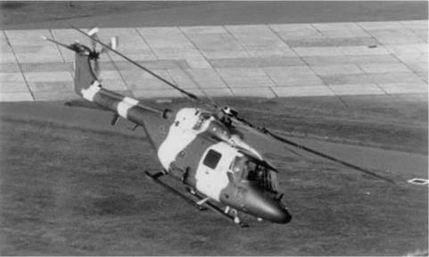
The SA 330 Puma is a twin-engine, medium-support helicopter in the 6-ton category, manufactured by Eurocopter France (ECF) (formerly Aerospatiale, formerly Sud Aviation), and in service with a number of civil operators and armed forces, including the Royal Air Force, to support battlefield operations. The DRA (RAE) research Puma XW241 (Fig. 4B.5) was one of the early development aircraft acquired by RAE in 1974 and extensively instrumented for flight dynamics and rotor aerodynamics research. With its original analogue data acquisition system, the Puma provided direct support during the 1970s to the development of new rotor aerofoils through the measurement of surface pressures on modified blade profiles. In
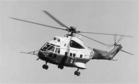
Fig. 4B.5 DRA research Puma XW241 in flight
|
Table 4B.3 Configuration data – Puma
|
the early 1980s a digital PCM system was installed in the aircraft and a research programme to support simulation model validation and handling qualities was initiated. Over the period between 1981 and 1988, more than 150 h of flight testing was carried out to gather basic flight mechanics data throughout the flight envelope of the aircraft (Ref. 4B.1). The aircraft was retired from RAE service in 1989.
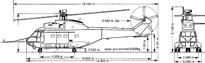
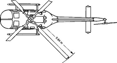
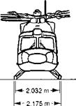
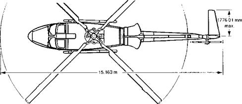
A three-view drawing of the aircraft in its experimental configuration is shown in Fig. 4B.6. The aircraft has a four-bladed articulated man rotor (modified NACA 0012 section, 3.8% flapping hinge offset). The physical characteristics of the aircraft used to construct the Helisim simulation model are provided in Table 4B.3.
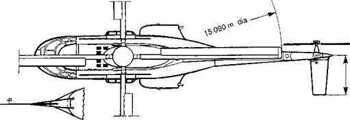
The Eurocopter Deutschland (formerly MBB) Bo105 is a twin engine helicopter in the 2.5-ton class, fulfilling a number of roles in transport, offshore, police and battlefield operations. The DLR Braunschweig operate two Bo105 aircraft. The first is a standard serial type (Bo105-S123), shown in Fig. 4B.3. The second aircraft is a specially modified fly – by-wire/light in-flight simulator – the ATTHEs (advanced technology testing helicopter system), Bo105-S3. The Bo105 features a four-bladed hingeless rotor with a key innovation for a 1960’s design – fibre-reinforced composite rotor blades.
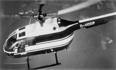
Fig. 4B.3 DLR research Bo105 S123 in flight
|
Table 4B.2 Configuration data – Bo105
|
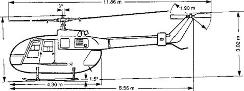
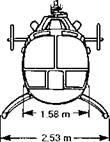
A three-view drawing of the aircraft is shown in a Fig. 4B.4, and the physical characteristics of the aircraft used to construct the Helisim simulation model are provided in Table 4B.2.
4B.1 Aircraft configuration parameters The DRA (RAE) research Lynx, ZD559
The Westland Lynx Mk 7 is a twin engine, utility/battlefield helicopter in the 4.5-ton category currently in service with the British Army Air Corps. The DRA Research Lynx (Fig. 4B.1) was delivered off the production line to RAE as an Mk 5 in 1985 and modified to Mk 7 standard in 1992. The aircraft is fitted with a comprehensive instrumentation suite and digital recording system. Special features include a strain-gauge fatigue usage monitoring fit, and pressure – and strain-instrumented rotor blades for fitment on both the main and tail rotor. The aircraft has been used extensively in a research programme to calibrate agility standards of future helicopter types. The four-bladed hingeless rotor is capable of producing
|
|
Fig. 4B.1 DRA research Lynx ZD559 in flight
|
Table 4B.1 Configuration data – Lynx
|
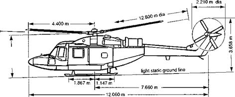
large control moments and hence angular accelerations. A 1960’s design, the Lynx embodies many features with significant innovation for its age – hingeless rotor with cambered aerofoil sections (RAE 9615, 9617), titanium monoblock rotor head and conformal gears.
A three-view drawing of the aircraft is shown in Fig. 4B.2. The physical characteristics of the aircraft used to construct the Helisim simulation model are provided in Table 4B.1.
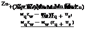
The application of Newton’s laws of motion to a helicopter in flight leads to the assembly of a set of nonlinear differential equations for the evolution of the aircraft response trajectory and attitude with time. The motion is referred to an orthogonal axes system fixed at the aircraft’s cg. In Chapter 3 we have discussed how these equations can be combined together in first-order vector form, with state vector x(t) of dimension n, and written as
x = F(x, u, t) (4A.1)
The dimension of the dynamic system depends upon the number of DoFs included. For the moment we will consider the general case of dimension n. The solution of eqn 4A.1 depends upon the initial conditions of the motion state vector and the time variation of the vector function F(x, u, t), which includes the aerodynamic loads, gravitational forces and inertial forces and moments. The trajectory can be computed using any of a number of different numerical integration schemes which time march through a simulation, achieving an approximate balance of the component accelerations with the applied forces and moments at every time step. While this is an efficient process for solving eqn 4A.1, numerical integration offers little insight into the physics of the aircraft flight behaviour. We need to turn to analytic solutions to deliver a deeper understanding between cause and effect. Unfortunately, the scope for deriving analytic solutions of general nonlinear differential equations as in eqn 4A.1 is extremely limited; only in special cases can functional forms be found and, even then, the range of validity is likely to be very small. Fortunately, the same is not true for linearized versions of eqn 4A.1, and much of the understanding of complex dynamic aircraft motions gleaned over the past 80 years has been obtained from studying linear approximations to the general nonlinear motion. Texts that provide suitable background reading and deeper understanding of the underlying theory of dynamic systems are Refs 4A.1-4A.3. The essence of linearization is the assumption that the motion can be considered as a perturbation about a trim or equilibrium condition; provided that the perturbations are small, the function F can usually be expanded in terms of the motion and control variables (as discussed earlier in this chapter) and the response written in the form
x = Xe + Sx (4A.2)
where Xe is the equilibrium value of the state vector and Sx is the perturbation. For convenience, we will drop the S and write the perturbation equations in the linearized form
x – Ax = Bu(t) + f(t) (4A.3)
where the (n x n) state matrix A is given by
and the (n x m) control matrix B is given by
and where we have assumed without much loss of generality that the function F is differentiable with all first derivatives bounded for bounded values of flight trajectory x and time t.
![]()
|
|||||||||||||||||||||||||||||||||||||||||||||||||
|
|||||||||||||||||||||||||||||||||||||||||||||||||
|
|||||||||||||||||||||||||||||||||||||||||||||||||
|
|||||||||||||||||||||||||||||||||||||||||||||||||
|
|||||||||||||||||||||||||||||||||||||||||||||||||
|
|||||||||||||||||||||||||||||||||||||||||||||||||
|
|||||||||||||||||||||||||||||||||||||||||||||||||
|
|
||||||||||||||||||||||||||||||||||||||||||||||||
|
|||||||||||||||||||||||||||||||||||||||||||||||||
|
|||||||||||||||||||||||||||||||||||||||||||||||||
|
|||||||||||||||||||||||||||||||||||||||||||||||||
|
|||||||||||||||||||||||||||||||||||||||||||||||||
|
|||||||||||||||||||||||||||||||||||||||||||||||||
|
|||||||||||||||||||||||||||||||||||||||||||||||||
|
|||||||||||||||||||||||||||||||||||||||||||||||||
|
of uncoupled equations
Уі – kyi = 0, i = 1, 2,…, n (4A.12)
with solutions
Уі = У^к‘ (4A.13)
Collected together in vector form, the solution can be written as
y = diag [exp (X, t)] У0 (4A.14)
Transforming back to the flight state vector x, we obtain
x(t) = W diag [exp (kit)] W-1×0 = Y(t)x0 = exp(At)x0 (4A.15)
where the principal matrix solution Y(t) is defined as
Y(t) = 0, t < 0, Y(t) = W diag [exp(X, t)] W-1, t > 0 (4A.16)
We need to stop here and take stock. The transformation matrix W and the set of numbers X have a special meaning in linear algebra; if wi is a column of W then the pairs [wi, Xi ] are the eigenvectors and eigenvalues of the matrix A. The eigenvectors are special in that when they are transformed by the matrix A, all that happens is that they change in length, as given by the equation
Aw і = Xi Wi (4A.17)
No other vectors in the space on which A operates are quite like the eigenvectors. Their special property makes them suitable as basis vectors for describing more general motion. The associated eigenvalues are the real or complex scalars given by the n solutions of the polynomial
det[XI – A] = 0 (4A.18)
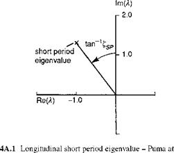
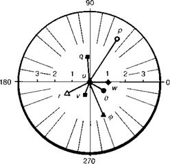
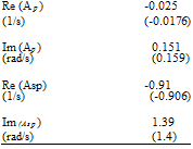
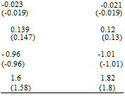
The free motion of a helicopter is therefore described by a linear combination of simple exponential motions, each with a mode shape given by the eigenvector and a trajectory envelope defined by the eigenvalue. Each mode is linearly independent of the others, i. e., the motion in a mode is unique and cannot be made up from a combination of other modes. Earlier in this chapter, a full discussion on the character of the modes of motion and how they vary with flight state and aircraft configuration was given. Below, in Figs 4A.1 and 4A.2, we illustrate the eigenvalue and eigenvector associated with the longitudinal short period mode of the Puma flying straight and level at 100 knots; we have included the modal content of all eight state vector components u, w, q, в, v, p, ф, r. The eigenvalue, illustrated in Fig. 4A.1, is given by
![]() Xsp = -1.0 ± 1.3i
Xsp = -1.0 ± 1.3i
 |
|
|
|
|
|
|
Fig. 4A.2 Longitudinal short period eigenvector – Puma at 100 knots |
The short period frequency is given by
asp = Im(ksp) = 1.3 rad/s (4A.21)
and, finally, the damping ratio is given by
zsp = – Re(Xsp) = 0.769 (4A.22)
asp
We choose to present the angular and translational rates in the eigenvectors shown in Fig. 4A.2 in deg/s and in m/s respectively. Because the mode is oscillatory, each component has a magnitude and phase and Fig. 4A.2 is shown in polar form. During the short period oscillation, the ratio of the magnitudes of the exponential envelope of the state variables remains constant. Although the mode is described as a pitch short period, it can be seen in Fig. 4A.2 that the roll and sideslip coupling content is significant, with roll about twice the magnitude of pitch. Pitch rate is roughly in quadrature with heave velocity.
 |
|
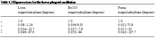
The eigenvectors are particularly useful for interpreting the behaviour of the free response of the aircraft to initial condition disturbances, but they can also provide key information on the response to controls and atmospheric disturbances. The complete solution to the homogeneous eqn 4A.3 can be written in the form
or expanded as
(4A.24)
where v is the eigenvector of the matrix AT, i. e., vT are the rows of W 1 (VT = W 1) so that
ATVj = X j Vj (4A.25)
The dual vectors w and v satisfy the bi-orthogonality relationship
vj Wk = 0, j = k (4A.26)
Equations 4A.24 and 4A.26 give us useful information about the system response. For example, if the initial conditions or forcing functions are distributed throughout the states with the same ratios as an eigenvector, the response will remain in that eigenvector. The mode participation factors, in the particular integral component of the solution, given by
vT(Bu(r) + f(r)) (4A.27)
determine the contribution of the response in each mode wi.
A special case is the solution for the case of a periodic forcing function of the form
f(t) = Fe‘ ю‘ = F (cos rnt + i sin rnt) (4A.28)
The steady-state response at the input frequency ю is given by
x(t) = X єіш‘
The frequency response function X is derived from the (Laplace) transfer function (of the complex variable s) evaluated on the imaginary axis. The transfer function for a given input (i )/output (o) pair can be written in the general form
![]() xo. s N(s)
xo. s N(s)
— (s) =——-
x D(s)
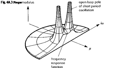
The response vector X is generally complex with a magnitude and phase relative to the input function F. Figure 4A.3 illustrates how the magnitude of the frequency response as a function of frequency can be represented as the value of the so-called transfer function,
when s = iЮ. In Fig. 4A.3 a single oscillatory mode is shown, designated the pitch short period. In practice, for the 6 DoF helicopter model, all eight poles would be present, but the superposition principle also applies to the transfer function. The peaks in the frequency response correspond to the modes of the system (i. e., the roots of the denominator D(s) = 0 in eqn 4A.30) that are set back in either the right-hand side or the left-hand side of the complex plane, depending on whether the eigenvalue real parts are positive (unstable) or negative (stable). The troughs in the frequency response function correspond to the zeros of the transfer function, or the eigenvalues for the case of infinite gain when a feedback loop between input and output is closed (i. e., the roots of the numerator N(s) = 0 in eqn 4A.30). Ultimately, at a high enough frequency, the gain will typically roll-off to zero as the order of D(s) is higher than N(s). The phase between input and output varies across the frequency range, with a series of ramp-like 180° changes as each mode is traversed; for modes in close proximity the picture is more complicated.
For the case when the system modes are widely separated, a useful approximation can sometimes be applied that effectively partitions the system into a series of weakly coupled subsystems (Ref. 4A.4). We illustrate the technique by considering the n-dimensional homogeneous system, partitioned into two levels of subsystem, with states x1 and x2, with dimensions I and m, such that n = I + m
![]()
![]() _Xi X2
_Xi X2
Equation 4A.31 can be expanded into two first-order equations and the eigenvalues can be determined from either of the alternative forms of characteristic equation
Л(*) = XI – A11 – AU(XI – A22)-1 A211 = 0 (4A.32)
Ж*) = XI – A22 – A21 (XI – An)-1 A12 = 0 (4A.33)
Using the expansion of a matrix inverse (Ref. 4A.4), we can write
![]()
 |
(XI – A22)-1 = – A-1 (I + XA221 + X2A-22 +—————————– )
We assume that the eigenvalues of the subsystems An |kjJ), kj2), and
A22|k2J 42), …, ї-f} are widely separated in modulus. Specifically, the eigenvalues of Aj j lie within the circle of radius r (r = max|kj!)|), and the eigenvalues of A22 lie without the circle of radius R (R = min|^2;’)|). We have assumed that the eigenvalues of smaller modulus belong to the matrix A jj. The method of weakly coupled systems is based on the hypothesis that the solutions to the characteristic eqn 4A.32 can be approximated by the roots of the first m + J terms and the solution to the characteristic eqn 4A.33 can be approximated by the roots of the last I + J terms, solved separately. It is shown in Ref. 4A.4 that this hypothesis is valid when two conditions are satisfied:
( J ) the eigenvalues form two disjoint sets separated as described above, i. e.,
[r] << J (4A.35)
(2) the coupling terms are small, such that if у and S are the maximum elements of the coupling matrices A 2 and A2 , then
When these weak coupling conditions are satisfied, the eigenvalues of the complete system can be approximated by the two polynomials
f1(*) = 1*1 – Aj J + Aj2 A—J A211 = 0 (4A.37)
f2W =|*I – A221 = 0 (4A.38)
According to eqns4A.37 and4A.38, the larger eigenvalue set is approximated by the roots of A22 and is unaffected by the slower dynamic subsystem AJJ. Conversely, the smaller roots, characterizing the slower dynamic subsystem AJJ, are strongly affected by the behaviour of the faster subsystem A22. In the short term, motion in the slow modes does not develop enough to affect the overall motion, while in the longer term, the faster modes have reached their steady-state values and can be represented by quasisteady effects.
 |
 |
|||||
The method has been used extensively earlier in this chapter, but here we provide an illustration by looking more closely at the longitudinal motion of the Puma helicopter in forward flight, given by the homogeneous form of eqn 4A.7, i. e.,
The eigenvalues of the longitudinal subsystem are the classical short period and phugoid modes with numerical values for the J00-knot flight condition given by
Phugoid: kJ>2 = —0.0Ю3 ± 0d76i (4A.40)
Short period: Л3 4 = —L0 ± L30i (4A.4J)
While these modes are clearly well separated in magnitude (r/R = O(0.2)), the form of the dynamic system given by eqn 4A.39 does not lend itself to partitioning as it stands. The phugoid mode is essentially an exchange of potential and kinetic energy, with excursions in forward velocity and vertical velocity, while the short period mode is a rapid incidence
adjustment with only small changes in speed. This classical form of the two longitudinal modes does not always characterize helicopter motion however; earlier in this chapter, it was shown that the approximation breaks down for helicopters with stiff rotors. For articulated rotors, the equations can be recast into more appropriate coordinates to enable an effective partitioning to be achieved. The phugoid mode can be better represented in terms of the forward velocity u and vertical velocity
w0 = w — Ue в (4A.42)
Equation 4A.39 can then be recast in the partitioned form
|
u |
Xu g cos 0e/Ue |
Xw — g cos 0e/Ue Xq — We |
u |
||
|
d |
w0 |
Zu g sin 0e/Ue |
Zw — g sin 0e/Ue Zq |
w0 |
|
|
dt |
w |
Zu g sin 0e/Ue |
Zw — g sin 0e/Ue Zq + Ue |
w |
|
|
. q. |
Mu 0 |
— 1 sf S3* |
q |
(4A.43)
The approximating polynomials for the phugoid and short period modes can then be derived using eqns 4A.37 and 4A.38, namely
Low-modulus phugoid (assuming Zq small):
 |
|||
(xw — UL cos 0^j (ZuMq — Mu (Zq + Ue))
High-modulus short period:
f2(k) = k2 — (Zw + Mq )k + Zw Mq — Mw (Zq + Ue) = 0 (4A.45)
A comparison of the exact and approximate eigenvalues is shown in Table 4A.1, using the derivatives shown in the charts of Appendix 4B. The two different ‘exact’ results are given for the fully coupled longitudinal and lateral equations and the uncoupled longitudinal set. Comparisons are shown for two flight speeds – 100 knots and 140 knots. A first point to note is that the coupling with lateral motion significantly reduces the phugoid damping,
|
Table 4A.1 Comparison of exact and approximate eigenvalues for longitudinal modes of motion
|
particularly at 140 knots where the oscillation is almost neutrally stable. The converse is true for the short period mode. The weakly coupled approximation fares much better at the higher speed and appears to converge towards the exact, uncoupled results. The approximations do not predict the growing loss of phugoid stability as a result of coupling with lateral dynamics, however. The higher the forward speed, the more the helicopter phugoid resembles the fixed – wing phugoid where the approximation works very well for aircraft with strongly positive manoeuvre margins (the constant term in eqn 4A.45 with negative Mw).
The approximations given by eqns 4A.44 and 4A.45 are examples of many that are discussed in Chapter 4 and that serve to provide additional physical insight into complex behaviour at a variety of flight conditions. The importance of the speed stability derivative Mu in the damping and frequency of the phugoid is highlighted by the expressions. For a low-speed fixed-wing aircraft, Mu is typically zero, while the effect of pitching moments due to speed effects dominates the helicopter phugoid. The last term in eqn 4A.45 represents the manoeuvre margin and the approximation breaks down long before instability occurs at positive values of the static stability derivative Mw (Ref. 4A.5).
To complete this appendix we present two additional results from the theory of weakly coupled systems. For cases where the system partitions naturally into three levels
|
A11 |
A12 |
A13 |
|
A21 |
A22 |
A23 |
|
A31 |
A32 |
A33 |
 |
![Подпись: leads to the low-order approximation /1(X) = det [XI — A11 + A12A—21(I + XA221)A21] (4A.50) Both these extensions to the more basic technique are employed in the analysis of Chapter 4.](/img/3131/image614.png) |
then the approximating polynomials take the form (see Ref. 4A.6)
Table 4.8 presents a comparison of the stability characteristics of Puma and Bo105 Helisim with flight estimates derived from the work of AGARD WG18 (Refs 4.22, 4.23). Generally speaking, the comparison of modal frequencies is very good, while dampings are less well predicted, particularly for the weakly damped or unstable phugoid and spiral modes. The pitch/heave subsidences for the Bo105 show remarkable agreement while the roll subsidence appears to be overpredicted by theory, although this is largely attributed to the compensating effect of an added time delay in the adopted model structure used to derive the flight estimates (Ref. 4.22). This aspect is returned to in Chapter 5 when results are
|
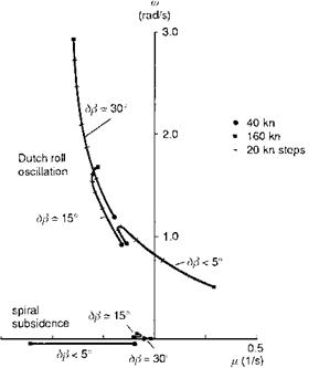
Fig. 4.29 Loci of Dutch roll and spiral mode eigenvalues with speed for different sideslip perturbations for Puma |
|
Table 4.8 Comparison of flight estimates and theoretical predictions of Puma and Bo105 stability characteristics
|
Shorthand notation:
X Complex variation ^ ± i&>;
[Z, o)n] damping ratio and natural frequency associated with roots of X2 + 2f&>„X + a>n2; (1/r) inverse of time constant т in root (X — 1 /т);
+Puma flight estimates from Glasgow/DRA analysis in Ref. 4.22;
++Bo105 flight estimates from DLR analysis in Ref. 4.22.
presented from the different model structures used for modelling roll response to lateral cyclic.
The above discussions have concentrated on 6 DoF motion analysis. There are several areas in helicopter flight dynamics where important effects are missed by folding the rotor dynamics and other higher order effects into the fuselage motions in quasi-steady form. These will be addressed in the context of constrained stability and aircraft response analysis in Chapter 5.
The lateral/directional motion of a helicopter in forward flight is classically composed of a roll/yaw/sideslip (Dutch roll) oscillation and two aperiodic subsidences commonly referred to as the roll and spiral modes. In hover, the modes have a broadly similar character, but different modal content. The roll subsidence mode is well characterized by the roll damping Lp at hover and, with some exceptions, throughout the speed envelope. The spiral mode in hover is largely made up of yaw motion (stability determined by yaw damping Nr) and the oscillatory mode could better be described as the lateral phugoid, in recognition of the similarity with the longitudinal phugoid mode already discussed. While the frequencies of the two hover oscillations are very similar, one big difference with the lateral phugoid is that the mode is predicted to be stable (for Bo105 and Lynx) or almost stable (Puma), on account of the strong contribution of yaw motion to the mode. The ratio of yaw to roll in this mode is typically about 2 for all three aircraft, rendering approximations based on a similar analysis to that conducted for the pitch phugoid unsuitable. We have to move into forward flight to find the Dutch roll mode more amenable to reduced order stability analysis, but even then there are complications that arise due to the roll/yaw ratio. For our case aircraft, the Lynx and Bo105 again exhibit similar characteristics to one another, while the Puma exhibits more individual behaviour, although not principally because of its articulated rotor. We shall return to the Puma later in this section, but first we examine the more conventional behaviour as typified by the Lynx.
Finding a suitable partitioning for approximating the lateral/directional modes requires the introduction of a new state variable into the lateral DoFs. With longitudinal motion we found that a partitioning into phugoid/short period subsets required the introduction of the vertical velocity, in place of the Euler pitch angle в. The basic problem is the same; where both the short period and phugoid involved excursions in w, both the spiral and Dutch roll mode typically involve excursions in the lateral velocity v as well as roll and yaw motion. However, it can be shown that the spiral mode is characterized by excursions in the sway
velocity component (Refs 4.12, 4.26)
(4.154)
In the derivation of this approximation we have extended the analysis to second-order terms (see Appendix 4A) to model the destabilizing effects of the dihedral effect shown in eqn 4.152.
Finally, the roll mode at the third level is given by
The accuracy of this set of approximations can be illustrated for the case of the Lynx at a forward flight speed of 120 knots, as shown below:
![]()
 Xsapprox — -0.039/s
2£dюdapprox — L32/s ^dapprox — 2-66 rad/s
Xrappoox — —10.3/s
The approximate eigenvalues are mostly well within 10% of the full subset predictions, which provides confidence in their worth, which actually holds good from moderate to high speeds for both Lynx and Bo105. The validity of this approximation for the Dutch roll oscillation depends upon the coupling between roll and yaw. The key coupling derivatives are Np and Lv, both of which are large and negative for our two hingeless rotor helicopters. The yaw due to roll derivative is augmented by the inertia coupling effects in eqn 4.48 (for the Lynx. Ixz — 2767 kg/m2; for the Bo105, Ixz — 660 kg/m2). The simplest approximation to the Dutch roll mode results when the coupling is zero so that the motion is essentially a yaw/sideslip oscillation. The yaw rate then exhibits a 90° phase lag relative to the sideslip and the damping is given by the first two terms in the numerator of eqn 4.152 (i. e., Nr + Yv). A negative value of Np tends to destabilize the oscillation by superimposing a roll motion into the mode such that the term Npp effectively adds negative damping. The eigenvector for the Dutch roll mode of the Lynx at 120 knots, shown below, illustrates that, while the yaw rate is still close to 90° out of phase with sideslip, the roll/yaw ratio is 0.5 with the yawing moment due to roll rate being almost in anti-phase with the sideslip.
v 1.0 m/s; p 0.02 rad/s (160°); r 0.04 rad/s (—80°)
The approximations described above break down when the roll/yaw ratio in the Dutch roll oscillation is high. Such a situation occurs for the Puma, and we close Chapter 4 with a discussion of this case.
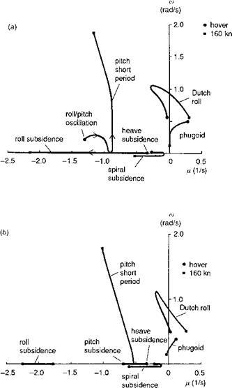
We refer back to Fig. 4.25(b) where the loci of the Puma eigenvalues are plotted with speed. Above 100 knots, the Dutch roll mode becomes less and less stable until at high speed the damping changes sign. At 120 knots, the Puma Dutch roll eigenvector is
v 1.0 m/s; p 0.04 rad/s (150°); r 0.01 rad/s (—70°)
which, compared with the Lynx mode shape, contains considerably more roll motion with a roll/yaw ratio of about 4, eight times that for the Lynx. The reason for the ‘unusual’
|
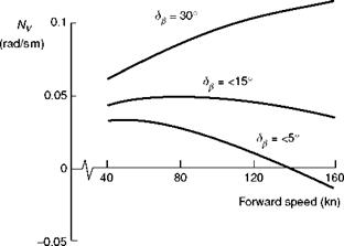
Fig. 4.28 Variation of weathercock stability derivative Nv with speed for different sideslip perturbations for Puma |
behaviour of the Dutch roll mode for the Puma can be attributed to the derivative Nv. In the previous discussion on this weathercock stability derivative, we observed that the Puma value was influenced by the strong nonlinearity in the force characteristics of the vertical fin with sideslip. At small angles of sideslip the fin sideforce is practically zero, due to the strong suction on the ‘undersurface’ of the thick aerofoil section (Refs 4.11,4.12). For larger angles of sideslip, the circulatory lift force builds up in the normal way. The value of the fin contribution to Nv therefore depends upon the amplitude of the perturbation used to generate the derivative (as with the yaw damping Nr, to a lesser extent). In Fig. 4.28, the variation of Nv with speed is shown for three different perturbation levels corresponding to <5°, 15° and 30° of sideslip. For the small amplitude case, the directional stability changes sign at about 140 knots and is the reason for the loss of Dutch roll stability illustrated in Fig. 4.25(b). For the large amplitude perturbations, the derivative increases with speed, indicating that the vertical fin is fully effective for this level of sideslip. Figure 4.29 presents the loci of Dutch roll eigenvalues for the three perturbation sizes as a function of speed, revealing the dramatic effect of the weathercock stability parameter. The mode remains stable for the case of the high sideslip perturbation level. It appears that the Puma is predicted to be unstable for small amplitudes and stable for large amplitude motion. These are classic conditions for so-called limit cycle oscillations, where we would expect the oscillation to limit in amplitude at some finite value with the mode initially dominated by roll and later, as the amplitude grows, to settle into a more conventional yaw/roll motion. We shall return to the nature of this motion when discussing response, in Chapter 5.
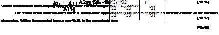
Hovering dynamics have long presented a challenge to reduced order modelling. The eigenvectors for the unstable hover ‘phugoid’ for the three aircraft are given in Table 4.3 and highlight that the contribution of the normal velocity w to this oscillation is less than 10% of the forward velocity u.
This suggests that a valid approximation to this mode could be achieved by neglecting the vertical motion and analysing stability with the simple system given by the surge and pitch equations
u — Xuu + gO — 0 (4.126)
q — Muu — Mqq — 0 (4.127)
The small Xq derivative has also been neglected in this first approximation. In vector – matrix form, this equation can be written as
![]()
![]() (4.128)
(4.128)
 |
|||
The partitioning has been added to indicate the approximating subsystems – the relatively high-frequency pitch subsidence and the low-frequency phugoid. Unfortunately, the first weakly coupled approximation indicates that the mode damping is given entirely by the derivative Xu, hence predicting a stable oscillation. We can achieve much better accuracy in this case by extending the analysis to the second approximation (see Appendix 4A), so that the approximating characteristic equation for the low-frequency oscillation becomes
The approximate phugoid frequency and damping are therefore given by the simple expressions
![]()
|
|
|
|
|
|
|
|
|
|
|
Fig. 4.26 Simple representation of unstable pitch phugoid in hover |
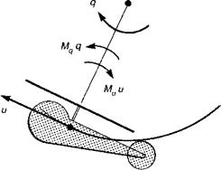
The ratio of the pitching moments due to speed (speed stability) and pitch rate (damping) play an important role in both the frequency and damping of the oscillation. This mode can be visualized in the form of a helicopter rotating like a pendulum about a virtual hinge (Fig. 4.26). The frequency of the pendulum is given by
a2 = 1 (4.133)
where t is the length of the pendulum (i. e., distance of helicopter centre of mass below the virtual hinge). This length determines the ratio of u to q in the eigenvector for this mode (cf. eqn 4.131). Comparison of the approximations given above with the ‘exact’ uncoupled phugoid roots is given in Table 4.4.
There is good agreement, particularly for the Lynx and Bo105. The smaller pitch damping for the Puma results in a more unstable motion, characteristic of articulated rotor helicopters at low speed. The speed stability derivative Mu is approximately proportional to the flapping derivative
дв1с 8
-Г1 =o °0 – 2^0 (4.134)
dp, 3
and scaled by the hub moment. The amount of flapback for a speed increment therefore depends only on the rotor loading, defined by the collective and inflow components. This derivative is the source of the instability and dominates the damping in eqn 4.132.
|
Table 4.4 Comparison of ‘exact’ and approximate hover phugoid eigenvalues
|
As the helicopter passes through the ‘trough’ of the oscillation, the velocity u and pitch rate q are both at a maximum, the former leading to an increased pitch-up, the latter leading to a pitch-down, which, in turn, leads to a further increase in the u velocity component. The strong coupling of these effects results in the conventional helicopter configuration always being naturally unstable in hover.
The concept of the helicopter oscillating like a pendulum is discussed by Prouty in Ref. 4.9, where the approximate expression for frequency of the motion is given by
![]()
![]() (4.135)
(4.135)
From eqn 4.133 we can approximate the location of the virtual point of rotation above the helicopter
The expression for the approximate damping given in eqn 4.132 provides a clue as to the likely effects of feedback control designed to stabilize this mode. The addition of pitch rate feedback (i. e., increase of Mq) would seem to be fairly ineffective and would never be able to add more damping to this mode than the natural source from the small Xu. Feeding back velocity, hence augmenting Mu, would appear to have a much more powerful effect; a similar result could be obtained through attitude feedback, hence adding effective derivatives Xв and Me.
The longitudinal pitch and heave subsidences hold no secrets at low speed and the eigenvalues are directly related to the damping derivatives in those two axes. The comparisons are shown in Table 4.5.
The hover approximations hold good for predicting stability at low speed, but in the moderate – to high-speed range, pitch and heave become coupled through the ‘other’ static stability derivative Mw, rendering the hover approximations invalid. From Figs 4.23(b), 4.24(b) and 4.25(b) we can see that the stability characteristics for the Lynx and Bo105 are quite different from that of the Puma. As might be expected, this is due to the different rotor types with the hingeless rotors exhibiting a much more unstable phugoid mode at high speed, while the articulated rotor Puma features a classical short – period pitch/heave oscillation and neutrally stable phugoid. At high speed, the normal velocity w features in both the long and short period modes and this makes it difficult to partition the longitudinal system matrix into subsystems based on the conventional aircraft states {u, w, q, в}. In Ref.4.25 it is shown that a more suitable partitioning can be found by recognizing that the motion in the long period mode is associated more
|
Table 4.5 Comparison of ‘exact’ and approximate longitudinal subsidences
|
with the vertical velocity component
w о = w — Ue8 (4.137)
Transforming the longitudinal equations into the new variables then enables a partitioning as shown in eqn 4.138:
|
u |
" Xu g cos 0e/Ue |
Xw — g cos 0e/Ue Xq — We" |
u |
|||
|
d |
w 0 |
Zu g sin 0e/Ue |
Zw — g sin 0e/Ue Zq |
w 0 |
||
|
dt |
w |
Zu g sin 0e/Ue |
Zw — g sin 0e/Ue Zq + Ue |
w |
||
|
. q. |
|_Mu 0 |
Mw Mq _ |
q |
(4.138)
Following the weakly coupled system theory in Appendix 4A, we note that the approximating characteristic equation for the low-frequency oscillation can be written as
X2 + 2Zp oip X + o/p — 0 (4.139)
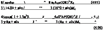
where the frequency and damping are given by the expressions (assuming Zq small and neglecting g sin ®e)
8
Xw — — cos 0e) (ZuMq — Mu(Zq + Ue))
![]()
![]() g „ rj Zw(ZuMq — Mu(Zq + Ue))
g „ rj Zw(ZuMq — Mu(Zq + Ue))
— cos 0^ Zu—————————————
Ue MqZw — Mw (Zq + Ue)
Similarly, the approximate characteristic equation for predicting the stability of the short period mode is given by
X2 + 2Ksp^spX + ^Sp = 0 (4.142)
where the frequency and damping are given by the expressions
2Ksp^sp = ~(Zw + Mq ) (4.143)
W2Sp — Zw Mq — (Zq + Ue)Mw (4.144)
The strong coupling of the translational velocities with the angular velocities in both short and long period modes actually results in the conditions for weak coupling being invalid for our hingeless rotor helicopters. The powerful Mu and Mw effects result in strong coupling between all the DoFs and the phugoid instability cannot be predicted using eqn 4.140. For the Puma helicopter, on the other hand, the natural modes are more classical, and very similar to a fixed-wing aircraft with two oscillatory modes becoming more widely separated as speed increases. Table 4.6 shows a comparison of the approximations for the phugoid
Table 4.6 Comparison of ‘exact’ and approximate longitudinal eigenvalues for Puma (exact results shown in parenthesis)
 |
 |
120 knots 140 knots 160 knots
and short period stability characteristics at high speed with the exact longitudinal subset results. The agreement is very good, particularly for the short period mode.
The short period mode involves a rapid incidence adjustment with little change in forward speed, and has a frequency of about 2 rad/s at high speed for the Puma. Increasing the pitch stiffness Mw increases this frequency. Key configuration parameters that affect the magnitude of this derivative are the tailplane effectiveness (moment arm x tail area x tail lift slope) and the aircraft centre of mass location. As noted in the earlier section on derivatives, the hub moment contribution to Mw is always positive (destabilizing), which accounts for the strong positive values for both Lynx and Bo105 and the associated major change in character of the longitudinal modes.
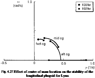 |
The significant influence of the aircraft centre of mass (centre of gravity (cg)) location on longitudinal stability is illustrated in Fig. 4.27, which shows the eigenvalue of the Lynx phugoid mode for forward (0.035 R), mid (0.0) and aft (-0.035 R) centre of mass locations as a function of forward speed. With the aft centre of mass, the mode has become severely unstable with a time to double amplitude of less than 1 s. At this condition the short period approximation, eqn 4.142, becomes useful for predicting this change in the stability
|
Table 4.7 Lynx stability characteristics with aft centre of mass
|
characteristics. The stiffness part of the short period approximation, given by eqn 4.144, is sometimes referred to as the manoeuvre margin of the aircraft (or the position of the aerodynamic centre relative to the centre of mass during a manoeuvre), and we can see from Table 4.7 that this parameter has become negative at high speed for the aft centre of mass case, due entirely to the strongly positive Mw. The divergence is actually well predicted by the short period approximation, along with the strong pitch subsidence dominated by the derivative Mq.
For small-amplitude stability analysis, helicopter motion can be considered to comprise a linear combination of natural modes, each having its own unique frequency, damping and distribution of the response variables. The linear approximation that allows this interpretation is extremely powerful in enhancing physical understanding of the complex motions in disturbed flight. The mathematical analysis of linear dynamic systems is summarized in Appendix 4A, but we need to review some of the key results to set the scene for the following discussion. Free motion of the helicopter is described by the homogeneous form of eqn 4.41
x – Ax = 0 (4.117)
subject to initial conditions
![]() x(0) = x0
x(0) = x0
The solution of the initial value problem can be written as
x(t) = W diag [exp(X;t)] W-1xo = Y(t)xo (4.119)
The eigenvalues, k, of the matrix A satisfy the equation
det[kI – A] = 0 (4.120)
and the eigenvectors w, arranged in columns to form the square matrix W, are the special vectors of the matrix A that satisfy the relation
Aw i = ki wi (4.121)
The solution can be written in the alternative form
n
x(t) = ^2(vTX0) exp(kit)wi (4.122)
i =0
where the v vectors are the eigenvectors of the transpose of A (columns of W-1), i. e.,
AT vj = k j vj (4.123)
The free motion is therefore shown in eqn 4.122 to be a linear combination of natural modes, each with an exponential character in time defined by the eigenvalue, and a distribution among the states, defined by the eigenvector.
The full 6 DoF helicopter equations are ninth order, usually arranged as [u, w, q, 9, v, р, ф,г, ф], but since the heading angle ф appears only in the kinematic equation relating the rate of change of Euler angle ф to the fuselage rates p, q, r, this equation is usually omitted for the purpose of stability analysis. Note that, for the ninth-order system including the yaw angle, the additional eigenvalue is zero (there is no aerodynamic or gravitational reaction to a change in heading) and the associated eigenvector is {0, 0, 0, 0, 0, 0, 0, 0, 1}.
The eight natural modes are described as linearly independent so that no single mode can be made up of a linear combination of the others and, if a single mode is excited precisely the motion will remain in that mode only. The eigenvalues and eigenvectors can be complex numbers, so that a mode has an oscillatory character, and such a mode will then be described by two of the eigenvalues appearing as conjugate complex pairs. If all the modes were oscillatory, then there would only be four in total. The stability of the helicopter can now be discussed in terms of the stability of the individual modes, which is determined entirely by the signs of the real parts of the eigenvalues. A positive real part indicates instability, a negative real part stability. As one might expect, helicopter handling qualities, or the pilot’s perception of how well a helicopter can be flown in a task, are strongly influenced by the stability of the natural modes. In some cases (for some tasks), a small amount of instability may be acceptable; in others it may be necessary to require a defined level of stability. Eigenvalues can be illustrated as points in the complex plane, and the variation of an eigenvalue with some flight condition or aircraft configuration parameter portrayed as a root locus. The eigenvalues are given as the solutions of the determinantal eqn 4.120, which can also be written in the alternate polynomial form as the characteristic equation
Xn + an—1Xn 1 +•••+ ai^i + ao = 0 (4.124)
or as the product of individual factors
(X – Xn)(X – Xn-)(……….. )(X – X1) = 0 (4.125)
The coefficients of the characteristic equation are nonlinear functions of the stability derivatives discussed in the previous section. Before we discuss helicopter eigenvalues and vectors, we need one further analysis tool that will prove indispensable for relating the stability characteristics to the derivatives.
Although eigenanalysis is a simple computational task, the eighth-order system is far too complex to deal with analytically, and we need to work analytically to glean any meaningful understanding. We have seen from the discussion in the previous section that many of the coupled longitudinal/lateral derivatives are quite strong and are likely to have a major influence on the response characteristics. As far as stability is concerned however, we shall make a first approximation that the eigenvalues fall into two sets – longitudinal and lateral, and append the analysis with a discussion of the effects of coupling. Even grouping into two fourth-order sets presents a formidable analysis problem, and to gain maximum physical understanding we shall strive to reduce the approximations for the modes even further to the lowest order possible. The conditions of validity of these reduced order modelling approximations are described in Appendix 4A where the method of weakly coupled systems is discussed (Ref. 4.24). In the present context the method is used to isolate, where possible, the different natural modes according to the dominant constituent motions. The partitioning works only when there exists a natural separation of the modes in the complex plane. Effectively, approximations to the eigenvalues of slow modes can be estimated by assuming that the faster modes behave in a quasi-steady manner. Likewise, approximations to the fast modes can be derived by assuming that the slower modes do not react in the fast time scale. A second condition requires that the coupling effects between the contributing motions are small. The theory is covered in Appendix 4A and the reader is encouraged to assimilate this before tackling the examples described later in this section.
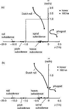
Figures 4.23, 4.24 and 4.25 illustrate the eigenvalues for the Lynx, Bo105 and Puma, respectively, as predicted by the Helisim theory. The pair of figures for each aircraft shows both the coupled longitudinal/lateral eigenvalues and the corresponding uncoupled values. The predicted stability characteristics of Lynx and Bo105 are very similar. Looking first at the coupled results for these two aircraft, we see that an unstable phugoid-type oscillation persists throughout the speed range, with time to double amplitude varying from about 2.5 s in the hover to just under 2 s at high speed. At the hover condition, this phugoid mode is actually a coupled longitudinal/lateral oscillation and is partnered by a similar lateral/longitudinal oscillation which develops into the classical Dutch roll oscillation in forward flight, with the frequency increasing strongly with speed. Apart from a weakly oscillatory heave/yaw oscillation in hover, the other modes are all subsidences having distinct characters at hover and low speed – roll, pitch, heave and yaw, but developing into more-coupled modes in forward flight, e. g., the roll/yaw spiral mode. The principal distinction between the coupled (Figs 4.23(a) and 4.24(a)) and the uncoupled (Figs 4.23(b) and 4.24(b)) cases lies in the
|
Fig. 4.23 Loci of Lynx eigenvalues as a function of forward speed: (a) coupled; (b) uncoupled |
stability of the oscillatory modes at low speed where the coupled case shows a much higher level of instability. This effect can be shown to be almost exclusively due to the coupling effects of the non-uniform inflow caused by the change in wake angle induced by speed perturbations; the important derivatives are Mv and Lu, caused by the coupled rotor flapping response to lateral and longitudinal distributions of first harmonic inflow respectively. The unstable mode is a coupled pitch/roll oscillation with similar ratios of p to q and v to u, in the eigenvector.
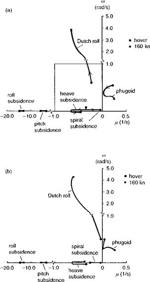
The Puma comparison is shown in Figs 4.25(a) and (b). The greater instability for the coupled case at low speed is again present, and now we also see the shortterm roll and pitch subsidences combined into a weak oscillation at low speed and hover. As speed increases the coupling effects again reduce, at least as far as stability is concerned. Here we are not discussing response and we should expect the coupled response characteristics to be strong at high speed, we shall return to this topic in the next chapter. At higher speeds the modes of the Puma, with its articulated rotor,
|
Fig. 4.24 Loci of Bo105 eigenvalues as a function of forward speed: (a) coupled; (b) uncoupled |
resemble the classical fixed-wing set: pitch short period, phugoid, Dutch roll, spiral and roll subsidence. An interesting feature of the Puma stability characteristics is the dramatic change in stability of the Dutch roll from mid- to high speed. We shall discuss this later in the section.
Apart from relatively local, although important, effects, the significance of coupling for stability is sufficiently low to allow a meaningful investigation based on the uncoupled results, and hence we shall concentrate on approximating the characteristics
|
Fig. 4.25 Loci of Puma eigenvalues as a function of forward speed: (a) coupled; (b) uncoupled |
illustrated in Figs 4.23(b)-4.25(b) and begin with the stability of longitudinal flight dynamics.
Of the 24 control derivatives, we have selected the 11 most significant to discuss in detail and have arranged these into four groups: collective force, collective moment, cyclic moment and tail rotor collective force and moment.
The derivatives Z00, Zви
 |
|
The derivative of thrust with main rotor collective and longitudinal cyclic can be obtained from the thrust and uniform inflow equations already introduced earlier in this chapter as eqns 4.66, 4.67. Approximations for hover and forward flight can be
From the derivative charts in the Appendix, Section 4B.2, it can be seen that this Z-force control derivative doubles in magnitude from hover to high-speed flight. This is the heave control sensitivity, and as with the heave damping derivative Zw, it is primarily influenced by the blade loading and tip speed. The reader is reminded that the force derivatives are in semi-normalized form, i. e., divided by the aircraft mass. The thrust sensitivity for all three case aircraft is about 0.15 g/° collective. Unlike the heave damping, the control sensitivity continues to increase with forward speed, reflecting the fact that the blade lift due to collective pitch changes divides into constant and two-per-rev components, while the lift due to vertical gusts is dominated by the one-per-rev incidence changes.
The thrust change with longitudinal cyclic is zero in the hover, and the approximation for forward flight can be written as
As forward speed increases, the change in lift from aft cyclic on the advancing blade is greater than the corresponding decrease on the retreating side, due to the differential dynamic pressure. As with the collective derivative at higher speeds, Ze1s increases almost linearly with speed, reaching levels at high speed very similar to the collective sensitivity in hover.
The derivatives M6o, Lво
Pitch and roll generated by the application of collective pitch arise from two physical sources. First, the change in rotor thrust (already discussed above) will give rise to a moment when the thrust line is offset from the aircraft centre of mass. Second, any change in flapping caused by collective will generate a hub moment proportional to the flap angle. It is the second of these effects that we shall focus on here. Referring to the flap response matrices from Chapter 3 (eqn 3.70), we can derive the main effect of collective pitch on flap by considering the behaviour of a teetering rotor at moderate forward speed. Hence we assume that
The aft flapping from increased collective develops from the greater increase in lift on the advancing blade, than on the retreating blade in forward flight. The effect grows in strength as forward speed increases, hence the approximate proportionality with speed. From the charts in the Appendix, Section 4B.2, we can observe that the effect is considerably stronger for the hingeless rotor configurations, as expected. In high-speed flight, the pitching moment from collective is of the same magnitude as the cyclic moment, illustrating the powerful effect of the differential loading from collective. Increasing collective also causes the disc to tilt to starboard (to port on the Puma). The physical mechanism is less obvious than for the pitching moment and according to the approximation in eqn 4.100, the degree of lateral flap for a change in collective pitch is actually a function of the rotor Lock number. The disc tilt arises from the rotor coning, which results in an increase in lift on the front of the disc and a decrease at the rear when the blades cone up (e. g., following an increase in collective pitch). The amount of lateral flapping depends on the coning, which itself is a function of the rotor Lock number. Once again, the resultant rolling moment will depend on the balance between thrust changes and disc tilt effects, which will vary from aircraft to aircraft (see control derivative charts in the Appendix, Section 4B.2).
The derivatives M01s, Mgu, Lвъ, Lвіс
The dominant rotor moments are proportional to the disc tilt for the centre-spring equivalent rotor and can be written in the form
Mr ~-(NTKe + hR^j etc, Lr «-(NbKp + hRT^j Plt (4.101)
The cyclic control derivatives can therefore be approximated by the moment coefficient in parenthesis multiplied by the flap derivatives. We gave some attention to these functions in Chapter 2 of this book. The direct and coupled flap responses to cyclic
|
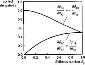
Fig. 4.22 Variation of rotor flap derivatives with Stiffness number |
control inputs are practically independent of forward speed and can be written in the form
where the Stiffness number is given by eqn 4.59. The variations of direct and crosscoupled flap derivatives with stiffness were illustrated in Fig. 2.21 (a), and are repeated here as Fig. 4.22 for the reader’s convenience. Up to Stiffness numbers of about 0.3 the direct flap derivative remains within a few percent of unity. The implication is that current so-called hingeless or ’semi-rigid’ rotors (e. g., Lynx and Bo105) flap in much the same way as a teetering rotor following a cyclic control input -1° direct flap for 1° cyclic. The cross-flap derivative arises with non-zero stiffness, because the natural frequency of flap motion is then less than one-per-rev, resulting in a flap response phase of less than 90°. The phase angle is given by tan-1 Sp, hence varying up to about 17° for Sp = 0.3. Although the cross-control derivative can be, at most, about 30% of the direct derivative, when considering pitch to roll coupling, this can result in a much greater coupled aircraft response to control inputs, because of the high ratio of pitch to roll inertias. This is evidenced by the coupling derivative Lq1s for the Lynx andBo105 in the charts of the Appendix, Section 4B.2, which is actually of higher magnitude than the direct control moment Me1s. The aircraft will therefore experience a greater initial roll than pitch acceleration following a step longitudinal cyclic input. The cyclic controls are usually ‘mixed’ at the swash plate partly to cancel out this initial coupling. We have already discussed the cross-coupling effects from pitch and roll rates and, according to the simple rotor theory discussed here, the total short-term coupling will be a combination of the two effects.
The derivatives Y6ot, Lвот, NgOT
According to the simple actuator disc model of the tail rotor, the control derivatives all derive from the change in tail rotor thrust due to collective pitch. As with the derivatives Nv and Nr, the control derivative also decreases by as much as 30% as a result of the action of a mechanical S3 hinge set to take off 1° pitch for every 1° flap. The exact value depends upon the tail rotor Lock number. In the derivative charts in the Appendix, Section 4B.2, we can see that the force derivative YeOT for the Bo105 is about 20% higher than the corresponding values for the Lynx and Puma. The Bo105 sports a teetering tail rotor so that the S3 effect works only to counteract cyclic flapping. The control derivatives increase with speed in much the same way as the main rotor collective Z-force derivative, roughly doubling the hover value at high speed as the V2 aerodynamics take effect.
The effects of non-uniform rotor inflow on damping and control derivatives
In Chapter 3 we introduced the concept of non-uniform inflow derived from local momentum theory applied to the rotor disc (see eqns 3.161, 3.181). Just as the uniform inflow balances the rotor thrust, so the flow needs to react to any hub moments generated by the rotor and a first approximation is given by a one-per-rev variation. The nonuniform inflow components can be written in the form given by
![]() x1c = (1 — C1) (ftc — ft* + q)
x1c = (1 — C1) (ftc — ft* + q)
ft* = (1 – C1) (01* – ftc + p)
where the lift deficiency factor in the hover takes the form
The non-uniform inflow has a direct effect on the flapping motion and hence on the moment derivatives. The effect was investigated in Refs 4.20 and 4.21 where a simple scaling of the rotor Lock number was shown to reflect the main features of the hub moment modification. We can write the flap derivatives as a linear combination of partial effects, as shown for the flap damping below:
![]() d^1c l Эв1Л Эв1с ЭА.1* Эв1с дХ1с
d^1c l Эв1Л Эв1с ЭА.1* Эв1с дХ1с
dq v dq Jut 9Л1* dq dX1c dq
The subscript ui indicates that the derivative is calculated with uniform inflow only. Using the expressions for the flap derivatives set down earlier in this section, we can write the corrected flap derivatives in the form
Se 16
P1cq = в1*р = g + ^ + Se C2 в1*9 (4.108)
P1*q = ~P1cp = g – SP^- SP C2 вЩ (4.109)
where the equivalent Lock number has been reduced by the lift deficiency factor, i. e.,
Y * = C1Y (4.110)
and the new C coefficient is given by the expression
![]()
(4.111)
Equation 4.108 shows the first important effect of non-uniform inflow that manifests itself even on rotors with zero hub stiffness. When the helicopter is pitching, the rotor lags behind the shaft by the amount given in eqn 4.108. This flapping motion causes an imbalance of moments which has a maximum and minimum on the advancing and retreating blades. This aerodynamic moment, caused by the flapping rate, gives rise to a wake reaction and the development of a non-uniform, laterally distributed component of downwash, к 1 s, serving to reduce the incidence and lift on the advancing and retreating blades. In turn, the blades flap further in the front and aft of the disc, giving an increased pitch damping Mq. The same arguments follow for rolling motion. The effect is quite significant in the hover, where the lift deficiency factor can be as low as 0.6.
By rearranging eqns 4.108 and 4.109, we may write the flap derivatives in the
 |
||
form
where the third C coefficient takes the form
and can be approximated by unity.
The new terms in parentheses in eqns 4.112 and 4.113 represent the coupling components of flapping due to the non-uniform inflow and can make a significant contribution to the lateral (longitudinal) flapping due to pitch (roll) rate, and hence to the coupled rate derivatives Lq and Mp.
A similar analysis leads to the control derivatives, which can be written in the forms
P1ce 1s —~P1se1C — – C3 (1 — C2Sj) (4.115)
fhce 1c — P1se 1s — C3 Cl (4.116)
C1
In the hover, for a rotor with zero flap stiffness, the aerodynamic moment due to flapping is exactly equal to that from the applied cyclic pitch; hence there is no non-uniform inflow in this case. The coupled flap/control response, given by eqn 4.116, is the only significant effect for the control moments indicating an increase of the coupled flapping of about 60% when the lift deficiency factor is 0.6.
Some reflections on derivatives
Stability and control derivatives aid the understanding of helicopter flight dynamics and the preceding qualitative discussion, supported by elementary analysis, has been
aimed at helping the reader to grasp some of the basic physical concepts and mechanisms at work in rotorcraft dynamics. Earlier in this chapter, the point was made that there are three quite distinct approaches to estimating stability and control derivatives: analytic, numerical, backward-forward differencing scheme and system identication techniques. We have discussed some analytic properties of derivatives in the preceding sections, and the derivative charts in the Appendix, Section 4B.3, illustrate numerical estimates from the Helisim nonlinear simulation model. A discussion on flight estimated values of the Bo105 and Puma stability and control derivatives is contained in the reported work of AGARD WG18 – Rotorcraft System Identification (Refs 4.22, 4.23). Responses to multistep control inputs were matched by 6 DoF model structures by a number of different system identification approaches. Broadly speaking, estimates of primary damping and control derivatives compared favourably with the Level 1 modelling described in this book. For cross-coupling derivatives and, to some extent, the lower frequency velocity derivatives, the comparisons are much poorer, however. In some cases this can clearly be attributed to missing features in the modelling, but in other cases, the combination of a lack of information in the test data and an inappropriate model structure (e. g., overparameterized model) suggests that the flight estimates are more in error. The work of AGARD WG18 represents a landmark in the application of system identification techniques to helicopters, and the reported results and continuing analysis of the unique, high-quality flight test data have the potential for contributing to significant increased understanding of helicopter flight dynamics. Selected results from this work will be discussed in Chapter 5, and the comparisons of estimated and predicted stability characteristics are included in the next section.
Derivatives are, by definition, one-dimensional views of helicopter behaviour, which appeal to the principle of superposition, and we need to combine the various constituent motions in order to understand how the unconstrained flight trajectory develops and to analyse the stability of helicopter motion. We should note, however, that superposition no longer applies in the presence of nonlinear effects, however small, and in this respect, we are necessarily in the realms of approximate science.
The direct and coupled damping derivatives are collectively one of the most important groupings in the system matrix. Primary damping derivatives reflect short-term, small and moderate amplitude, handling characteristics, while the cross-dampings play a dominant role in the level of pitch-roll and roll-pitch couplings. They are the most potent derivatives in handling qualities terms, yet because of their close association with short-term rotor stability and response, they can also be unreliable as handling parameters. We shall discuss this issue later in Chapter 5 and in more detail in Chapter 7, but first we need to explore the many physical mechanisms that make up these derivatives. There has already been some discussion on the roll damping derivative in Chapter 2, when some of the fundamental concepts of rotor dynamics were introduced. The reader is referred back to the Tour (Section 2.3) for a refresher.
Taking the pitch moment as our example for the following elucidation, we write the rotor moment about the centre of mass in the approximate form
Mr = — Nb Ke + Th^j flic (4.81)
where Kp is the flapping stiffness, T the rotor thrust and h r the rotor vertical displacement from the centre of mass. In this simple analysis we have ignored the moment due to the in-plane rotor loads, but we shall discuss the effects of these later in this section. The rotor moment therefore has two components – one due to the moment of the thrust vector tilt from the centre of mass, the other from the hub moment arising from real or effective rotor stiffness. Effective stiffness arises from any flap hinge offset, where the hub moment is generated by the offset of the blade lift shear force at the flap hinge. According to eqn 4.81, the rotor moment is proportional to, and hence in phase with, the rotor disc tilt (for the centre-spring rotor). The relative contributions of the two components depend on the rotor stiffness. The hub pitch moment can be expanded in the form (see eqns 3.104, 3.105)
Mh = ~NbKep1c = – N & lp (k2p – 1) P1c (4.82)
and the corresponding roll moment as
Lh = – NbKjep1s = –2 & Ip (k} – 1) P1s (4.83)
The hub moment derivatives can therefore be derived directly from the flapping derivatives. Since the quasi-steady assumption indicates that the disc tilt reaches its steady – state value before the fuselage begins to move, the flap derivatives can be obtained from the matrix in eqn 3.72; thus, in hover, where the flap effects are symmetrical,
|
Эв1с |
dft1s |
1 |
(So + Y) |
(4.84) |
|
d q |
9 p |
1 + Se |
||
|
dfitc |
dPs |
1 |
(Se 7 – 0 |
(4.85) |
|
9 p |
d q |
1 + Se |
The Stiffness number Sp is given by eqn 4.59.
The variation of the flap damping derivatives in eqns 4.84 and 4.85 with the fundamental stiffness and Lock parameters has been discussed in Chapter 2 (see Figs 2.21 (b) and (c)). For values of Stiffness number up to about 0.4, corresponding to the practical limits employed in most current helicopters, the direct flap derivative is fairly constant, so that helicopters with hingeless rotors flap in very much the same way as helicopters with teetering rotors. The Lock number has a much more dramatic effect on the direct flap motion. Looking at the coupling derivatives, we can see a linear variation over the same range of Stiffness number, with rotors having low Lock number experiencing a reversal of sign. This effect is manifested in the Bo105 helicopter, as illustrated in the derivative charts of the Appendix, Section 4B.2, where the Lock number of 5 and Stiffness number of about 0.4 result in a practical cancelling of the rolling moment due to pitch rate Lq. The rotor Lock number is critically important to the degree of pitch-roll coupling.
From the theory of flap dynamics derived in Chapter 3, we can explain the presence of the two terms in the flap derivatives. The primary mechanism for flap and rotor damping derives from the second term in parenthesis in eqn 4.84 and is caused by the aerodynamic moment generated by the flapping rate (at azimuth positions 90° and 270°) that occurs when the rotor is pitching. The disc precesses as a result of the aerodynamic action at these azimuth stations, and lags behind the rotor shaft by the angle (16/уй) x pitch rate. The primary mechanism for coupling is the change in one-per-rev aerodynamic lift generated when the rotor pitches or rolls (second term in eqn 4.85), adding an effective cyclic pitch. Both effects are relatively insensitive to changes in rotor stiffness. The additional terms in Sp in eqns 4.84 and 4.85 arise from the fact that the flap response is less than 90° out of phase with the applied aerodynamic load. The direct aerodynamic effects, giving rise to the longitudinal and lateral flapping, therefore couple into the lateral and longitudinal flapping respectively. The effect on the coupling is especially strong since the direct flap derivative provides a component in the coupling sense through the sign of the phase angle between aerodynamic load and flap response.
Combining the flap derivatives with the hub moments in eqns 4.82 and 4.83, we can derive approximate expressions for the rotor hub moment derivatives, in seminor – malized form, for small values of Sp:
The hub moment derivatives are therefore scaled by the Stiffness number, but otherwise follow the same behaviour as the flap derivatives. They also increase with blade number and rotorspeed. It is interesting to compare the magnitude of the hub moment with the thrust tilt contribution to the rotor derivatives. For the Lynx, the hub moment represents about 80% of the total pitch and roll damping. For the Puma, the fraction is nearer 30% and the overall magnitude is about 25% of that for the Lynx. Such is the powerful effect of rotor flap stiffness on all the hub moment derivatives reflected in the values of Sp for the Lynx and Puma of 0.22 and 0.044 respectively. As can be seen from the derivative charts in the Appendix, Section 4B.2, except for the pitch damping, most of the rate derivatives discussed above are fairly constant over the speed range, reflecting the insensitivity with forward speed of rotor response to equivalent cyclic pitch change. The pitch damping derivative Mq also has a significant stabilizing contribution from the horizontal tailplane, amounting to about 40% of the total at high speed.
 |
|
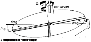
Before leaving the roll and pitch moment derivatives, it is important that we consider the influence of the in-plane rotor loads on the moments transmitted to the fuselage. In our previous discussion of the force derivatives Xq and Yp, we have seen how the ‘Amer effect’ reduces the effective rotor damping, most significantly on teetering rotors in low-thrust flight conditions. An additional effect stems from the orientation of the in-plane loads relative to the shaft when the rotor disc is tilted with one-per-rev flapping. The effect is illustrated in Fig. 4.21, showing the component of rotor torque oriented as a pitching moment with lateral flapping (the same effect gives a rolling moment with longitudinal flapping). The incremental hub moments can be written in terms of the product of the steady torque component and the disc tilt; hence, for four-bladed rotors
Fig. 4.21 Source of rotor hub couple due to inclination of rotor torque to the shaft
These moments will then combine with the thrust vector tilt and hub moment to give the total rotor moment. To examine the contribution of all three effects to the derivatives, we compare the breakdown for the Puma and Lynx. The Helisimpredicted hover torque for the Puma and Lynx work out at about 31 000 N m and 18000 N m respectively. The corresponding rotor thrusts are 57 000 N and 42 000 N and the effective spring stiffnesses 48 000 N m/rad and 166 000 N m/rad. The resultant derivative breakdown can then be written in the form
![]()
Lynx
![]() дв1с dB1s дв1с dB1s
дв1с dB1s дв1с dB1s
Mp = -6.62— + 0.46— Mp = -27.82— + 0.66—
p d p dp p dp d p
The effect of the torque moment on the direct damping derivative is therefore negligible. In the case of the coupling derivative, the effect appears to be of concern only for articulated rotors, and then only for rotors with very light blades (see the low Lock number cases in Figs 2.21(b) and (c)).
The derivatives Nr, Lr, Np
The final set of rate derivatives have little in common in terms of their physical makeup but share, along with their ‘big brother’ Lp, the property of having a primary influence on the character of the lateral/directional stability and control characteristics of the helicopter. We begin with a discussion of the yaw damping derivative Nr. In our previous discussion of the force derivatives, we rather dismissed the sideforce due to yaw rate Yr, since the inertial effect due to forward speed (Uer) was so dominating. The aerodynamic contribution to Yr, however, is directly linked to the yaw damping and is dominated by the loads on the tail rotor and vertical fin. Assuming that these components are at approximately the same location, we can write the yaw damping as
Nr ~ – It-r^Yr (4.94)
hz
In the hover, our theory predicts that Nr is almost entirely due to the tail rotor, with a numerical value of between -0.25 and -0.4, depending on the tail rotor design parameters, akin to the effect of main rotor design parameters on Zw (see Table 4.2). The low value of yaw damping is reduced even further (by about 30%) by the effect of the mechanical S3 coupling built into tail rotors to reduce transient flapping. The fin ‘blockage’ effects on the tail rotor can reduce Nr by another 10-30% depending on the separation and relative cover of the tail rotor from the fin. Yaw motion in the hover is therefore very lightly damped with a time constant of several seconds.
In low-speed manoeuvres the effect of the main rotor downwash over the tail boom can have a strong effect on the yaw damping. The flow inclination over the tail boom can give rise to strong circulatory loads for deep, slender tail booms. This effect has been explored in terms of tail rotor control margins in sideways flight (Refs 4.9, 4.16 and 4.17), and the associated tail boom loads in steady conditions, from which we
can deduce the kind of effects that might be expected in manoeuvres. The magnitude of the moment from the sideloads on the tail boom in a yaw manoeuvre depends on a number of factors, including the strength and distribution of main rotor downwash, the tail boom ‘thickness ratio’ and the location of any strakes to control the flow separation points (Ref. 4.16). A fixed strake, located to one side of the tail boom (for example, to reduce the tail rotor power requirement in right sideways flight), is likely to cause significant asymmetry in yaw manoeuvres. Main rotors with low values of static twist will have downwash distributions that increase significantly towards the rotor tips, leading to a tail boom centre of pressure in manoeuvres that is well aft of the aircraft centre of mass. The overall effect is quite complex and will depend on the direction of flight, but increments to the yaw damping derivative could be quite high, perhaps even as much as 100%.
As forward speed increases, so does the yaw damping in an approximately proportional way up to moderate speeds, before levelling off at high speed, again akin to the heave damping on the main rotor. The reduced value of Nr for the Puma, compared with Lynx and Bo105, shown in Appendix 4B, stems from the low fin effectiveness at small sideslip angles discussed earlier in the context of the weathercock stability derivative Nv. For larger sideslip excursions the derivative increases to the same level as the other aircraft.
One small additional modifying effect to the yaw damping is related to the rotor – speed governor sensing a yaw rate as an effective change in rotorspeed. At low forward speeds, the yaw rate can be as high as 1 rad/s, or between 2 and 4% of the rotorspeed. This will translate into a power change, hence a torque change and a yaw reaction on the fuselage serving to increase the yaw damping, with a magnitude depending on the gain and droop in the rotorspeed governor control loop.
Np and Lr couple the yaw and roll DoFs together. The rolling moment due to yaw rate has its physical origin in the vertical offset of the tail rotor thrust and vertical fin sideforce from the aircraft centre of mass. Lr should therefore be positive, with the tail rotor thrust increasing to starboard as the aircraft nose yaws to starboard. However, if the offsets are small and the product of inertia Ixz relatively high, so that the contribution of Nr to Lr increases, Lr can change sign, a situation occurring in the Lynx, as shown in the derivative charts of the Appendix, Section 4B.2. The derivative Np is more significant and although the aerodynamic effects from the main and tail rotor are relatively small, any product of inertia Ixz will couple the roll into yaw with powerful consequences. This effect can be seen most clearly for the Lynx and Bo105 helicopters. The large negative values of Np cause an adverse yaw effect, turning the aircraft away from the direction of the roll (hence turn). In the next section we shall see how this effect influences the stability characteristics of the lateral/directional motion. Before leaving Np and the stability derivatives however, it is worth discussing the observed effect of large torque changes during rapid roll manoeuvres (Refs 4.18, 4.19). On some helicopters this effect can be so severe that overtorquing can occur and the issue is given attention in the cautionary notes in aircrew manuals. The effect can be represented as an effective Np. During low – to moderate-amplitude manoeuvres, the changes in rotor torque caused by the drag increments on the blades are relatively benign. However, as the roll rate is increased, the rotor blades can stall, particularly when rolling to the retreating side of the disc (e. g., a roll rate of 90o/s will generate a local incidence change of about 3o at the blade tip). The resulting transient rotor torque change can now be significant and lead to large demands on the engine. The
situation is exacerbated by the changes in longitudinal flapping and hence pitching moment with roll rate as the blades stall. Within the structure of the Level 1 Helisim model, this effect cannot be modelled explicitly; a blade element rotor model with nonlinear aerodynamics is required. The nonlinear nature of the phenomenon, to an extent, also makes it inappropriate to use an equivalent linearization, particularly to model the onset of the effect as roll rate increases.