Category HELICOPTER FLIGHT DYNAMICS

In Chapter 2 we discussed the mechanism of cyclic pitch, cyclic flapping and the re­sulting hub moments generated by the tilt of the rotor disc. In Chapters 3 and 4, the aeromechanics associated with cyclic flapping was modelled in detail. In this section, we build on this extensive groundwork and examine features of the attitude response to cyclic pitch, chiefly with the Helisim Bo105 as a reference configuration. Simulated re­sponses have been computed using the full nonlinear version of Helisim with the control inputs at the rotor ($1s and 01c), and are presented in this form, unless otherwise stated.

Response to step inputs in hover – general features

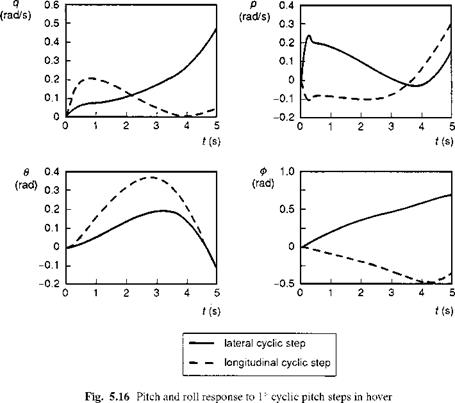
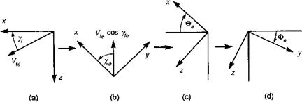
Figure 5.16 shows the pitch and roll response to 1° cyclic step inputs at the hover. It can be seen that the direct response after 1s, i.e., q to 01s and p to 01c, has a similar magnitude

for both pitch and roll – in the present case about 12°/s per deg of cyclic. However, while the hub moments and rate sensitivities (i. e., the steady-state rate response per degree of cyclic) are similar, the control sensitivities and dampings are scaled by the respective inertias (pitch moment of inertia is more than three times the roll moment of inertia). Thus the maximum roll rate response is achieved in about one-third the time it takes for the maximum pitch rate to be reached. The short-term cross-coupled responses (q and

p) exhibit similar features, with about 40% of the corresponding direct rates (p and

q) reached less than 1 s into the manoeuvre. The accompanying sketches in Fig. 5.17 illustrate the various influences on the helicopter in the first few seconds of response from the hover condition. The initial snatch acceleration is followed by a rapid growth to maximum rate when the control moment and damping moment effectively balance. The cross-coupled control moments are reinforced by the coupled damping moments in the same time frame. As the aircraft accelerates translationally, the restoring moments due to surge and sway velocities come into play. However, these effects are counteracted by cross-coupled moments due to the development of non-uniform induced velocities normal to the rotor disc (A. is and A. ic). After only 3-4 s, the aircraft has rolled to nearly 30° following either pitch or roll control inputs, albeit in opposite directions. Transient motion from the hover is dominated by the main rotor dynamics and aerodynamics. In the very short time scale (<1 s), the attitude response is strongly influenced by the rotor flapping dynamics and we need to examine this effect in more detail.

Effects of rotor dynamics

The rotor theory of Chapter 3 described three forms of the multi-blade coordinate representation of blade flap motion – quasi-steady, first-and second order. Figure 5.18 compares the short-term response with the three different rotor models to a step lateral cyclic input in hover. The responses of all three models become indistinguishable after about 1 s, but the presence of the rotor regressing flap mode (Bo105 frequency approximately 13 rad/s – see Chapter 4) is most noticeable in the roll rate response in the first quarter of a second, giving rise to a 20% overshoot compared with the deadbeat response of the quasi-steady model. The large-scale inset figure shows the comparison over the first 0.1s, highlighting the higher order dynamic effects, including the very fast dynamics of the advancing flap mode in the second-order representation. With rotor dynamics included, the maximum angular acceleration (hence hub moment) occurs after about 50 ms, or after about 120° rotor revolution for the Bo105. The quasi­steady approximation, which predicts the maximum hub moment at t = 0, is therefore valid only for low-frequency dynamics (below about 10 rad/s). We have already seen earlier in this chapter how rotor dynamics have a profound effect on the stability of the rotor/fuselage modes under the influence of strong attitude control. This is a direct result of the effective time delay caused by the rotor transient shown in Fig. 5.18. Unless otherwise stated, the examples shown in this section have been derived using the first-order rotor flap approximation.

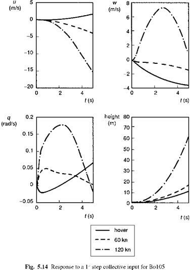
The response to collective in forward flight is considerably more complicated than in hover. While collective pitch remains the principal control for vertical velocity and flight path angle up to moderate forward speed, pilots normally use a combination of collective and cyclic to achieve transient flight path changes in high-speed flight. Also, collective pitch induces powerful pitch and roll moments in forward flight. Figure 5.14

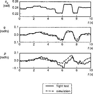
compares the longitudinal response of the Helisim Bo105 to collective steps in hover, at 60 and 120 knots. Comparisons are made between perturbations in forward velocity u, heave velocity w, pitch rate q and height h. We draw particular attention to the comparison of the w – velocity component and the relationship with climb rate. In hover, the aircraft reaches its steady rate of climb of about 4 m/s (750 ft/min) in about 5 s. At 120 knots the heave velocity component is initially negative, but almost immediately reverses and increases to about 7 m/s in only 3 s. The height response shows that the aircraft has achieved a climb rate of 20 m/s (approx. 3800 ft/min) after about 4 s. The powerful pitching moment generated by the collective input (M$0), together with the pitch instability (Mw), has caused the aircraft to zoom climb, achieving a pitch rate of about 10°/s after only 2 s. Thus, the aircraft climbs while the heave velocity (climb rate, V9) increases positively. The pitching response due to collective is well predicted by our Level 1 Helisim model as shown in Fig. 5.15, which compares flight and simulation for

the Bo105 excited by a collective (modified) 3211 input at 80 knots. The 3211 test input, in standard and modified forms, was developed by the DLR (Ref. 5.14) as a general – purpose test input with a wide frequency range and good return to trim properties. Figure 5.15 compares the pitch and roll response to the collective disturbance. Roll response is less well predicted than pitch, with the simulated amplitude only 50% of the flight measurement, although the trends are correct. The roll response will be largely affected by the change in main rotor incidence in the longitudinal plane, caused by elastic coning, pitch rate and non-uniform inflow effects; the Helisim rigid blade approximation will not, of course, simulate the curvature of the blade.

In this first example, we examine in some detail the apparently straightforward case of a helicopter’s vertical response to collective in hover. In both Chapters 2 and 4 we have already discussed the quasi-steady approximation for helicopter vertical motion given by the first-order equation in vertical velocity

w – Zww = Ze0 00 (5.52)

where the heave damping and control sensitivity derivatives are given from momentum theory in terms of the blade loading Ma /Ab, tip speed Й and hover-induced velocity Xo (or thrust coefficient Ct), by the expressions (see Chapter 4)

A comparison of the vertical acceleration response to a collective step input derived from eqn 5.52 with flight measurements on the DRA research Puma is shown in Fig. 5.10. It can be seen that the quasi-steady model fails to capture some of the detail in the response shape in the short term, although the longer term decay is reason­ably well predicted. For low-frequency collective inputs, the quasi-steady model is expected to give fairly high fidelity for handling qualities evaluations, but at moderate to high frequencies, the fidelity will be degraded. In particular, the transient thrust peaks observed in response to sharp collective inputs will be smoothed over. The sig­nificance of this effect was first examined in detail by Carpenter and Fridovitch in the

early 1950s, in the context of the performance characteristics of rotorcraft during jump take-offs (Ref. 5.17). Measurements were made of rotor thrust following the application of sharp and large collective inputs and compared with results predicted by a dynamic rotor coning/inflow nonlinear simulation model. The thrust changes T were modelled by momentum theory, extended to include the unsteady effects on an apparent mass of air mam, defined by the circumscribed sphere of the rotor.

dv; 2 / 2 de

T = mam — + 2n R2p vAvi – w + 3 R — (5.55)

where

4 3

mam = 0.637p—n R3 (5.56)

In eqn 5.55 we have added the effect of aircraft vertical motion w, not included in the test stand constraints in Ref. 5.17; v; is the induced velocity and в the blade flapping. Thrust overshoots of nearly 100% were measured and fairly well predicted by this relatively simple theory, with the inflow build-up, as simulated by eqn 5.55, accounting for a significant proportion of this effect. A rational basis for this form of inflow modelling and the associated azimuthal non-uniformities first appeared in the literature in the early 1970s, largely in the context of the prediction of hub moments (Ref. 5.18), and later with the seminal work of Pitt and Peters in Ref. 5.19. The research work on dynamic inflow by Pitt and Peters, and the further developments by Peters and his co-workers, has already received attention in Chapters 3 and 4 of this book. Here we observe that Ref. 5.19 simulated the rotor loading with a linear combination of polynomial functions that satisfied the rotor blade tip boundary conditions and also satisfied the underlying unsteady potential flow equation. The Carpenter-Fridovitch apparent mass approximation was validated by Ref. 5.19, but a ‘corrected’ and reduced value was proposed as an alternative that better matched the loading conditions inboard on the rotor.

Based on the work of Refs 5.17 and 5.19, an extensive analysis of the flight dynamics of helicopter vertical motion in hover, including the effects of aircraft motion, rotor flapping and inflow, was conducted by Chen and Hindson and reported in Ref. 5.20. Using a linearized form of eqn 5.55 in the form

ST = mamVi + 2nR2 pj2ko(2vi – w) + 3RgJ (5.57)

Chen and Hindson predicted the behaviour of the integrated 3 DoF system and pre­sented comparisons with flight test data measured on a CH-47 helicopter. The large transient thrust overshoots were confirmed and shown to be strong functions of rotor trim conditions and Lock number. The theory in Ref. 5.20 was developed in the con­text of evaluating the effects of rotor dynamics on the performance of high-gain digital flight control, where dynamic behaviour over a relatively wide frequency range would potentially affect the performance of the control system. One of the observations in Ref. 5.20 was related to the very short-term effect of blade flapping on the fuselage response. Physically, as the lift develops on a rotor blade, the inertial reaction at the hub depends critically on the mass distribution relative to the aerodynamic centre. For the case where the inertial reaction at the hub is downward for an increased lift, the aircraft
normal acceleration to collective pitch transfer function will exhibit a so-called non­minimum phase characteristic; although the eventual response is in the same direction as the input, the initial response is in the opposite direction. One of the consequences of very-high-gain feedback control with such systems is instability. In practice, the gain level necessary to cause concern from this effect is likely to be well outside the range required for control of helicopter vertical motion.

An extensive comparison of the behaviour of the Chen-Hindson model with flight test data was conducted by Houston on the RAE research Puma in the late 1980s and reported in Refs 5.16, 5.21-5.23, and we continue this case study with an exposition of Houston’s research findings. They demonstrate the utility of applied system identification, and also highlight some of the ever-present pitfalls. The linearized derivative equations of motion for the 3 DoF – vertical

The blade Lock number and hover value of inflow are given by the expressions

The expressions for the Z derivatives indicate that the resultant values are determined by the difference between two inertial effects of similar magnitude. Accurate estimates of the mass moments are therefore required to obtain fidelity in the heave DoF. In Houston’s analysis the rotorspeed was assumed to be constant, a valid approximation for short-term response modelling. In Ref. 5.24, results are reported that include the effects of rotorspeed indicating that this variable can be prescribed in the above 3 DoF model with little loss of accuracy.

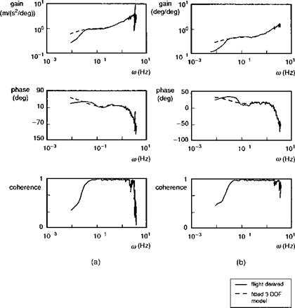
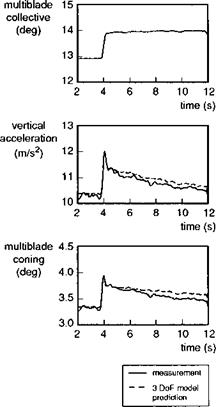
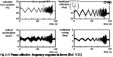
Flight tests were conducted on the Puma to measure the vertical motion and rotor coning in response to a collective frequency sweep. Figure 5.11 shows a sample of the test data with collective lever, rotor coning angle (derived from multi-blade coordinate analysis) andnormal acceleration at the aircraft centre of mass (Ref. 5.21). The test input was applied over a wide frequency range from less than 0.1 Hz out to 3.5 Hz. The test data were converted to the frequency domain using fast Fourier transform techniques for transfer function modelling. Figure 5.12 shows an example of the magnitude, phase and coherence of the acceleration and coning response along with the fitted 3 DoF model, derived from a least-squares fit of magnitude and phase. The coherence function indicates strong linearity up to about 2 Hz with some degradation up to about 3 Hz, above which the coherence collapses. The increasing response magnitude in both heave and coning DoFs is a characteristic of the effects of inflow dynamics. The identified model parameters and modal stability characteristics are shown in Table 5.2, compared with the theoretical predictions for the Puma using the derivative expressions in eqns 5.59-5.62. The percentage spread gives the range of values estimated from six different sets of test data.

Key observations from the comparisons in Table 5.2 are that theory predicts the inflow derivatives reasonably accurately but overestimates the coning derivatives by over 30%; the heave derivatives are typically of opposite sign and the predicted stability

is considerably greater than that estimated from flight. In an attempt to reconcile these differences, Houston examined the effects of a range of gross model ‘corrections’ based on physical reasoning of both aerodynamic and structural effects, but effectively distorting the derivatives in eqns 5.59-5.62. Close examination of Houston’s analysis shows that two of the correction factors effectively compensated for each other, hence resulting in somewhat arbitrary final values. We can proceed along similar lines by noting that each of the derivative groups – inflow, coning and heave – have similar errors in the theoretical predictions, suggesting that improved theoretical predictions may be obtained for each group separately. Considering the inflow derivatives, we can see that the inflow/collective derivative is predicted to within 2% of the flight estimate. This gives confidence in the Carpenter-Fridovitch value of the apparent mass coefficient Co. The other key parameter in eqn 5.59 is the hover value of rotor inflow. An empirical correction factor of 0.7 applied to this value, together with a 2% reduction in Co, leads to the modified theoretical estimates given in Table 5.2, now all within 10% of the flight values. The coning derivatives are a strong function of blade Lock number as shown in eqn 5.60; a 30% reduction in blade Lock number from 9.37 to 6.56, brings

the coning derivatives all within 5% of the flight values, again shown in Table 5.2. The heave derivatives are strongly dependent on the inertia distribution of the rotor blade as already discussed. We can see from eqn 5.61 that the heave due to coning is proportional to the first mass moment M p. Using this simple relation to estimate a corrected value for M p, a 30% reduction from 300 to 200 kg m2 is obtained. The revised values for the heave derivatives are now much closer to the flight estimates as shown in Table 5.2, with the heave damping within 15% and control sensitivity within 4%. The application of model parameter distortion techniques in validation studies gives an indication of the extent of the model deficiencies. The modified rotor parameters can be understood qualitatively in terms of several missing effects – non-uniform inflow, tip and root losses, blade elasticity and unsteady aerodynamics, and also inaccuracies in the estimates of blade structural parameters. For the present example, the correction consistency across the full set of parameters is a good indication that the modifications are physically meaningful.

The example does highlight potential problems with parameter identification when measurements are deficient; in the present case, no inflow measurements were available and the coherence of the frequency response functions was seen to decrease sharply above about 3 Hz, which is where the coning mode natural frequency occurs (see Table 5.2). The test data are barely adequate to cover the frequency range of interest in the defined model structure and it is remarkable how well the coning mode charac­teristics are estimated. In the time domain, the estimated 3 DoF model is now able to reflect much of the detail missed by the quasi-steady model. Figure 5.13 illustrates a comparison of time responses of coning and normal acceleration following a 1° step in collective pitch. The longer term mismatch, appearing after about 5 s, is possibly due to the effects of unmodelled rotorspeed changes. In the short term, the transient flapping and acceleration overshoots are perfectly captured. The significance of these

higher order modelling effects has been confirmed more recently in a validation study of the Ames Genhel simulation model with flight test data from a UH-60 helicopter in hovering flight (Ref. 5.25).

The RAE research reported by Houston was motivated by the need for robust criteria for vertical axis handling qualities. At that time, the international effort to develop new handling qualities standards included several contending options. In the event, a simple model structure was adopted for the low-frequency control strategies required in gross bob-up type manoeuvres. This topic is discussed in more detail in Section 6.5. For high-gain feedback control studies however, a 3 DoF model should be used to address the design constraints associated, for example, with very precise height keeping.

5.3.1 General

Previous sections have focused on trim and stability analysis. The analysis of flight behaviour following control or disturbance inputs is characterized under the general heading ‘Response’, and is the last topic of this series of modelling sections. Along with the trim and stability analysis, response forms a bridge between the model build­ing activities in Chapter 3 and the flying qualities analysis of Chapters 6 and 7. In the following sections, results will be presented from so-called system identification techniques, and readers unfamiliar with these methods are strongly encouraged to de­vote some time to familiarizing themselves with the different tools (Ref. 5.14). Making sense of helicopter dynamic flight test data in the validation context requires a com­bination of experience (e. g., knowing what to expect) and analysis tools that help to isolate cause and effect, and hence provide understanding. System identification methods provide a rational and systematic approach to this process of gaining better understanding.

Before proceeding with a study of four different response topics, we need to recall the basic equations for helicopter response, given in earlier chapters and Appendix 4A. The nonlinear equations for the motion of the fuselage, rotor and other dynamic elements, combined into the state vector x(t), in terms of the applied controls u(t) and disturbances f(t), can be written as

dx, ,

dt = F(x(t), u(t), f(t); t)

with solution as a function of time given by

t

x(t) = x(0) + y F(x(r), u(t), f(r); т)dr (5.48)

0

In a forward simulation, eqn 5.48 is solved numerically by prescribing the form of the evolution of F(t) over each time interval and integrating. For small enough time intervals, a linear or low-order polynomial form for F(t) generally gives rapid conver­gence. Alternatively, a process of prediction and correction can be devised by iterating on the solution at each time step. The selection of which technique to use will usually not be critical. Exceptions occur for systems with particular characteristics (Ref. 5.15), leading to premature numerical instabilities, largely determined by the distribution of eigenvalues; inclusion of rotor and other higher order dynamic modes in eqn 5.47 can sometimes lead to such problems and care needs to be taken to establish a sufficiently robust integration method, particularly for real-time simulation, when a constraint will be to achieve the maximum integration cycle time. We will not dwell on these clearly important issues here, but refer the reader to any one of the numerous texts on numerical analysis.

The solution of the linearized form of eqn 5.47 can be written in either of two forms (see Appendix 4A)

t

x(t) = Y(t)x0 + f Y(t – r )(Bu(t ) + f(r)) dr (5.49)

0

n t –

(t) = ^2 (vTX0) exp(V) + f (vt(Bu(t) + f(r)) exp[X;(t – r)]) dr

i=1 L "

(5.50)

where the principal matrix solution Y(t) is given by

Y(t) = 0, t < 0, Y(t) = W diag[exp(^t)]VT, t > 0 (5.51)

W is the matrix of right-hand eigenvectors of the system matrix A, VT = W-1 is the matrix of eigenvectors of AT, and X( are the corresponding eigenvalues; В is the control matrix. The utility of the linearized response solutions depends on the degree of nonlinearity and the input and response amplitude. In general terms, the linear formulation is considerably more amenable to analysis, and we shall regularly use linear approximations in the following sections to gain improved understanding. In particular, the ability to estimate trends through closed-form analytic solutions, exploited fully in the analysis of stability, highlights the power of linear analysis and, unless a nonlinearity is obviously playing a significant role, equivalent linear systems analysis is always preferred in the first instance.

It is inevitable that the following treatment has to be selective; we shall examine response characteristics in different axes individually, concerning ourselves chiefly with direct response to controls. In several cases, comparisons between flight and He – lisim simulation are shown and reference is made to the AGARD Working Group 18 (Rotorcraft System Identification) flight test databases for the DRA Puma and DLR Bo105 helicopters (Ref. 5.14).

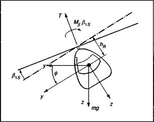
We consider a simple model of a helicopter being flown along a prescribed flight path in two-dimensional, horizontal flight (Fig. 5.7). The key points can be made with the most elementary simulation of the helicopter flight dynamics (i. e., quasi-steady rotor dynamics). It is assumed that the pilot is maintaining height and balance with collective and pedals, respectively. The equation for the rolling motion is given in terms of the lateral flapping Ps:

IxxФ = ~Mp Pis (5.35)

where Mp is the rolling moment per unit flapping given by

Mp = (+ hRT) (5.36)

The rotor thrust T varies during the manoeuvre to maintain horizontal flight. As de­scribed in Chapter 3, the hub stiffness Kp can be written in terms of the flap frequency ratio Xp, flap moment of inertia Ip and rotorspeed Й, in the form

Kp = (k2p – l) (5.37)

The equations of force balance in earth axes can be written as

T cos (ф – Pis) = mg (5.38)

T sin (ф – Pis) = my (5.39)

where y(t) is the lateral flight path displacement. Combining eqns 5.35, 5.38 and 5.39, and assuming small roll and lateral flapping angles (including constant rotor thrust), we obtain the second-order equation for the roll angle ф

Where v is the normalized sideforce (i. e., lateral acceleration) given in linearized form by

v = y/g (5.4l)

and the ‘natural’ frequency оц is related to the rotor moment coefficient by the expres­sion

(5.42)

The rotor and fuselage roll time constants are given in terms of more fundamental rotor parameters, the rotor Lock number (y) and the roll damping derivative (Lp)

The reader should note that the assumption of constant frequency оф implies that the thrust changes are small compared with the hub component of the rotor moment. The frequency Оф is equal to the natural frequency of the roll-regressive flap mode

discussed in Chapters 2 and 4.

Equation 5.40 holds for general small amplitude lateral manoeuvres and can be used to estimate the rotor forces and moments, hence control activity, required to fly a manoeuvre characterized by the lateral flight path y(t). This represents a simple case of so-called inverse simulation (Ref. 5.13), whereby the flight path is prescribed and the equations of motion solved for the loads and controls. A significant difference between rotary and fixed-wing aircraft modelled in this way is that the inertia term

in eqn 5.40 vanishes for fixed-wing aircraft, with the sideforce then being simply proportional to the roll angle. For helicopters, the loose coupling between rotor and fuselage leads to the presence of a mode, with dynamics described by eqn 5.40, with frequency шф, representing an oscillation of the aircraft relative to the rotor, while the rotor maintains the prescribed orientation in space. We have already seen evidence of a similar mode in the previous analysis of constrained vertical motion. Oscillations of the fuselage in this mode, therefore, have no effect on the flight path of the aircraft. It should be noted that this ‘mode’ is not a feature of unconstrained flight, where the two natural modes are a roll subsidence (magnitude Lp) and a neutral mode (magnitude 0), representing the indifference of the aircraft dynamics to heading or lateral position. The degree of excitation of the ‘new’ free mode depends upon the frequency content of the flight path excursions and hence the sideforce v. For example, when the prescribed flight paths are genuinely orthogonal to the free oscillation (i. e., combinations of sine waves), then the response will be uncontaminated by the free oscillation. In practice, slalom-type manoeuvres, while similar in character to sine waves, can have significantly different load requirements at the turning points, and the scope for excitation of the free oscillation is potentially high. A further important point to note about the character of the solution to eqn 5.40 is that as the frequency of the flight path approaches the natural frequency шф, the roll angle approaches a ‘resonance’ condition. To understand what happens in practice, we must look at the equation for ‘forward’ rather than ‘inverse’ simulation. This can be written in terms of the lateral cyclic control input Qc forcing the flight path sideforce v, in the approximate form

The derivation of this equation depends on the assumption that the rotor responds to control action and fuselage angular rate in a quasi-steady manner, taking up a new disc tilt instantaneously. In reality the rotor responds with a time constant equal to (16/y Й), but for the purposes of the present argument this delay will be neglected. The presence of the control acceleration term on the right-hand side of eqn 5.44 is crucial to what happens close to the natural frequency. In the limit, when the input frequency is at the natural frequency, the flight path response is zero due to the cancelling of the control terms, hence the implication of the theoretical artefact, in eqn 5.40, that the roll angle would grow unbounded at that frequency. As the pilot moves his stick at the critical frequency, the rotor disc remains horizontal and the fuselage wobbles beneath. We found a similar effect for longitudinal motion. For cyclic control inputs at slightly lower frequencies, the sideforces are still very small and large control displacements are required to generate the turning moments. Stick movements at frequencies slightly higher than шф produce small forces of the opposite sign, acting in the wrong direction. Hence, despite intense stick activity the pilot may not be able to fly the desired track. The difference between what the pilot can do and what he is trying to do increases sharply with the severity of the desired manoeuvre, and the upper limit of what can usefully or safely be accomplished, in terms of task ‘bandwidth’, is determined by the frequency шф. For current helicopters, the natural frequency шф varies from 6 rad/s for low hinge offset, slowly rotating rotors, to 12 rad/s for hingeless rotors with higher rotor speeds.

Two questions arise out of the above simple analysis. First, as the severity of the task increases, what influences the cut-off frequency beyond which control activity becomes unreasonably high and hence can this cut-off frequency be predicted? Second, how does the pilot cope with the unconstrained oscillations, if indeed they manifest themselves in practice. A useful parameter in the context of the first question is the ratio of aircraft to task natural frequencies. The task natural frequency can, in general, be derived from a frequency analysis of the flight path variation, but for simple slalom manoeuvres the value is approximately related to the inverse of the task time. It is suggested in Ref. 5.12 that a meaningful upper limit to task frequency can be written in the form

^ > 2nv (5.45)

&t

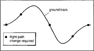
where nv is the number of flight path changes required in a given task. A two-sided slalom, for example, as illustrated in Fig. 5.8, contains five such distinct changes; hence at a minimum, for slalom manoeuvres

Ют

-т> 10 (5.46)

This suggests that a pilot flying a reasonably agile aircraft, with юф = 10 rad/s, could be expected to experience control problems when trying to fly a two-sided slalom in less than about 6 s. A pilot flying a less agile aircraft (юф = 7 rad/s) might experience similar control problems in a 9-s slalom. This 50% increase in usable performance for an agile helicopter clearly has very important implications for military and some civil operations.

Figures 5.9(a)-(c) show results from an inverse simulation of Helisim Lynx fitted with different rotor types flying a slalom mission task element (Ref. 5.12). Three rotor configurations are shown on the figures corresponding to юф = 11.8 (standard Lynx), юф = 7.5 (articulated) and юф = 4.5 (teetering). The aspect ratio of the slalom, defined as the overall width to length, is 0.077, the maximum value achievable by the teetering rotor configuration before the lateral cyclic reaches the control limits; the flight speed is 60 knots. Figures 5.9(a) and (b) show comparisons of the roll attitude and rate responses respectively. The attitude changes, not surprisingly, are very similar for the three cases,

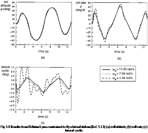
as are the rates, although we can now perceive the presence of higher frequency motion in the signal for the teetering and articulated rotors. For the teetering rotor, roll rate peaks some 10 – 20% higher than required with the hingeless rotor can be observed – entirely a result of the component of the free mode in the aircraft response. Figure 5.9(c) illustrates the lateral cyclic required to fly the 0.077 slalom, the limiting aspect ratio for the teetering configuration. The extent of the excitation of the roll oscillation for the different cases, and hence the higher frequency ‘stabilization’ control inputs, is shown clearly in the time histories of lateral cyclic. The difference between the three rotor configurations is now very striking. The Lynx, with its standard hingeless rotor, requires 30% of maximum control throw, while the articulated rotor requires slightly more at about 35%.

In Ref. 5.12, the above analysis is extended to examine pilot workload metrics based on control activity. The premise is that the conflict between guidance and stabi­lization is a primary source of workload for pilots as they attempt to fly manoeuvres beyond the critical aircraft/task bandwidth ratio. Both time and frequency domain workload metrics are discussed in Ref. 5.12, and correlation between inverse simu­lation and Lynx flight test results is shown to be good; the limiting slalom for both cases was about 0.11. This line of research to determine reliable workload metrics for

predicting critical flying qualities boundaries is, in many ways, still quite formative, and detailed coverage, in this book, of the current status of the various approaches is therefore considered to be inappropriate.

The topic of stability under constraint is an important one in flight dynamics, and the examples described in this section have illustrated how relatively simple anal­ysis, made possible by certain sensible approximations, can sometimes expose the physical nature of a stability boundary. This appears fortuitous but there is actually a deeper underlying reason why these simple models work so well in predicting prob­lems. Generally, the pilot will fly a helicopter using a broad range of control inputs, in terms of both frequency and amplitude, to accomplish a task, often adopting a control strategy that appears unnecessarily complex. There is some evidence that this strat­egy is important for the pilot to maintain a required level of attention to the flying task, and hence, paradoxically, plentiful spare capacity for coping with emergencies. Continuous exercise of a wide repertoire of control strategies is therefore a sign of a healthy situation with the pilot adopting low to moderate levels of workload to stay in command. A pilot experiencing stability problems, particularly those that are self­induced, will typically concentrate more and more of his or her effort in a narrow frequency range as he or she becomes locked into what is effectively a man-machine limit cycle. Again paradoxically, these very structured patterns of activity in pilot con­trol activity are usually a sign that handling qualities are deteriorating and workload is increasing.

Consider helicopter flight where the pilot is using the cyclic or collective to maintain constant vertical velocity w0 = w — Ue9. In the case of zero perturbation from trim, so that the pilot holds a constant flight path, we can write the constraint in the form

w = Ue9 (5.21)

When the aircraft pitches, the flight path therefore remains straight. We can imagine control so strong that the dynamics in the heave axis is described by the simple algebraic relation

Zuu + Zww ~ 0 (5.22)

and the dynamics of surge motion is described by the differential equation

du g

——– Xuu + — w = 0 (5.23)

dt Ue J

In this constrained flight, heave and surge velocity perturbations are related through the ratio of heave derivatives; thus

Zu

w ^———- – u (5.24)

Zw

and the single unconstrained degree of surge freedom is described by the first-order system

The condition for speed stability can therefore be written in the form

Xu + < 0 (5.26)

Ue Zw

For the Lynx, and most other helicopters, this condition is violated below about 60 knots as the changes in rotor thrust with forward speed perturbations become more and more influenced by the strong changes in rotor inflow. Hence, whether the pilot

applies cyclic or collective to maintain a constant flight path below approximately min­imum power speed, there is a risk of the speed diverging unless controlled. In practice, the pilot would normally use both cyclic and collective to maintain speed and flight path angle at low speed. At higher forward speeds, while the speed mode is never well damped, it becomes stable and is dominated by the drag of the aircraft (derivative Xu). At steep descent angles the control problems become more acute, as the vertical response to both collective and cyclic reverses, i. e., the resulting change in flight path angle following an aft cyclic or up collective step is downward (Refs 5.10, 5.11).

Strong control of the aircraft flight path has an even more powerful influence on the pitch attitude modes of the aircraft, which also change character under vertical motion constraint. Consider the feedback control between vertical velocity and longitudinal cyclic pitch, given by the simple proportional control law

01s = kw0 w 0 (5.27)

Rearranging the longitudinal system matrix in eqn 4.138 to shift the heave (w0) variable to the lowest level (i. e., highest modulus) leads to the modified system matrix, with partitioning as shown, namely

The damping in the low-modulus speed mode is approximated by the expression

and we note that as the feedback gain increases, the stability becomes asymptotic to the value given by the simpler approximation in eqn 5.26. If we make the reasonable assumptions

then the condition for stability is given by the expression

For the Lynx at 40 knots, a gain of 0.35°/(m/s) would be sufficient to destabilize the speed mode.

The approximation for the mid-modulus pitch ‘attitude’ mode is given by the expression

where we have used the additional approximations

Mels » UeMw (5.33)

Zeu * UeZw (5.34)

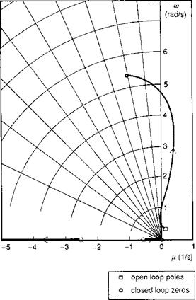
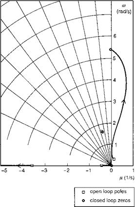
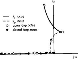
In the form of eqn 5.32, the approximation is therefore able to estimate only the location of the pitch mode at infinite gain. The mode is predicted to be stable, with a damping given by the pitch damping derivative and frequency by the pitch control sensitivity derivative. The mode has the appearance of a pendulum mode, with the fuselage rocking beneath the rotor, the latter remaining fixed relative to the flight path. An obvious question that arises from the above analysis relates to how influential this mode is likely to be on handling qualities and, hence, what the character of the mode is likely to be at lower values of gain. Figure 5.5 shows the root loci for the 3 DoF longitudinal modes of the Lynx at a 60 knots level flight condition. The locus near the origin is the eigenvalue of the speed mode already discussed, with the closed-loop zero at the origin (neutral stability). The root moving out to the left on the real axis corresponds to the strongly controlled vertical mode. The finite zero, characterizing the pitch mode,

is shown located where approximate theory predicts, with a damping ratio of about 0.2. Of particular interest is the locus of this root as the feedback gain is increased, showing how, for a substantial range of the locus (up to a gain of approximately unity), the mode is driven increasingly unstable. This characteristic is likely to inhibit strong control of the flight path in the vertical plane far more than the loss of stability in the speed mode.

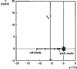
The moderately high frequency of the pitch mode at high values of gain suggests that there is the potential for coupling with the regressing flap mode. Figure 5.6 illus­trates the same root loci for the 9 DoF Lynx model; the lower level oscillatory root on Fig. 5.6 represents the Dutch roll oscillation. The roll regressing mode is not shown on the axes range, but is actually hardly affected by the control. What does happen is that the pitch mode now becomes neutrally stable in the limit, with correspondingly more significant excursions into the unstable range at lower values of gain. Even when the open-loop pole has been stabilized through pitch attitude and rate feedback, we can expect the same general trend, with instability occurring at relatively low values of gain. The physical source of the instability is the reduction in incidence stability (Mw) resulting from the control of vertical velocity with cyclic pitch; a positive change

in incidence will indicate an increased rate of descent and will be counteracted by a positive (aft) cyclic, hence reducing static stability. A more natural piloting strategy is to use collective for flight path control and cyclic for speed and attitude control. At low to moderate speeds this strategy will always be preferred, and sufficient collective margin should be available to negate any pilot concerns not to over-torque the ro – tor/engine/transmission. At higher speeds however, when the power margins are much smaller, and the flight path response to cyclic is stronger, direct control of flight path with cyclic is more instinctive. The results shown in Figs 5.5 and 5.6 suggest a poten­tial conflict between attitude control and flight path control in these conditions. If the pilot tightens up the flight path control (e. g., air-to-air refuelling or target tracking), then a PIO might develop. We have already seen evidence of PIOs from the analysis of strong attitude control in the last section. Both effects are ultimately caused by the loose coupling between rotor and fuselage and are inherently more significant with helicopters than with fixed-wing aircraft. PIOs represent a limit to safe flight for both types of aircraft and criteria are needed to ensure that designs are not PIO prone. This issue will be addressed further in Chapter 6.

The examples discussed above have highlighted a conflict between attitude control (or stability) and flight path control (or guidance) for the helicopter pilot. This conflict is most vividly demonstrated by an analysis of constrained flight in the horizontal plane (Ref. 5.12).

To illustrate the principal effects of strong attitude control, we first examine pitch control and simplify the analysis by considering the longitudinal subset only. The essential features are preserved under this decoupled approximation. Strong control is assumed to be applied by the pilot or SCAS through simple proportional and rate feedback of pitch attitude to the longitudinal cyclic pitch

6s = кев + kqq, ke, kq < 0 (5.1)

where the gains к are measured in deg/deg (deg/deg s) or rad/rad (rad/rad s). Typi­cal values used in limited authority SCAS systems are 0(0.1), whereas pilots can adopt gains an order of magnitude greater than this in tight tracking tasks. We make the assumption that, for high values of gain, the pitch attitude в and rate q, motions separate off from the flight path translational velocities u and w, leaving these latter variables to dominate the unconstrained modes. This line of argument leads to a partitioning of the longitudinal system matrix (subset of eqn 4.45) in the form

The derivatives have now been augmented by the control terms as shown. Before deriving the approximating polynomials for the low modulus (u, w) and high mod­ulus (0, q) subsystems, we note that the transfer function of the attitude response to longitudinal cyclic can be written in the form

0(s) (Ug + ke)R(s) (5 3)

01s(s) = D(s) ( . )

where the polynomial D(s) is the characteristic equation for the longitudinal open-loop eigenvalues. The eigenvalues of the closed-loop system are given by the expression

D(k) — (kkg + ke) R(k) = 0

where the polynomial R(k) gives the closed-loop zeros, or the eigenvalues for infinite control gains, and can be written in the expanded form

R(k) = k2 — ^Xu + Zw — m— (MuX01s + MwZ01s)^J к

+ ( XuZw — ZuXw + —— (Xe1s (ZuMw — MuZw) + Ze1s (MuXw — MwXu)) )

M01s /

(5.5)

Equation 5.5 signifies that there are two finite zeros for strong attitude control and, referring to eqn 5.4, we can see a further zero at the origin for strong control of pitch rate. Figure 5.1 shows a sketch of the loci of longitudinal eigenvalues for variations in ke and kg. The forms of the loci are applicable to hingeless rotor configurations, which exhibit two damped aperiodic modes throughout the speed range. Articulated rotor helicopters, whose short-term dynamics are characterized by a short period oscillation, would exhibit a similar pattern of zeros. The two finite zeros shared by both the attitude and rate control loops are given by the roots of eqn 5.5 and both remain stable over the forward flight envelope. For strong control, we can derive approximations for the closed-loop poles of the augmented system matrix in eqn 5.2 from the weakly coupled

approximations to the low- (unconstrained motion) and high (constrained motion) order subsystems, as defined by the partitioning shown in eqn 5.2. The general form of the approximating quadratic is written as

k2 + 2^rnk + a>2 = 0 (5.6)

For the low-order subsystem, we can write

2z® = — (Xu + Zw ——— (MuXe1s + MwZe1s +—

V M$1s V ke

*2 = (XuZw — ZuXw + Mbiifa — t)

X( ZuMw — MuZw ) + Ze1s (MuXw — MwXu)N)^)

and for the high-order subsystem

k2 — (Mq + kqMe1s) k — keMe1s = 0 (5.9)

The approximations work well for moderate to high levels of feedback gain (k 0(1)). For weak control (k O(0.1)) however, the approximations given above will not produce accurate results. To progress here we should have to derive an analytic extension to the approximations for the open-loop poles derived in Chapter 4. The terms in eqns 5.7 and 5.8 that are independent of the control derivatives reflect the crude, but effective, approximation found by perfectly constraining the pitch attitude. The two subsidences of the low-order approximation, which emerge from strong attitude control, are essentially a speed mode (dominated by u), with almost neutral stability, and a heave mode (dominated by w), with time to half amplitude given approximately by the heave damping Zw. The strongly controlled mode, with stability given by eqn 5.9, exhibits an increase in frequency proportional to the square root of attitude feedback gain, and in damping proportional to the rate feedback gain. The shift of the (open-loop) pitch and heave modes to (closed-loop) heave and speed modes at high gain is accompanied by a reduction in the stability of these flight trajectory motions, but the overall coupled aircraft/controller system remains stable.

A concern with strong attitude control is actually not so much with the uncon­strained motion, but rather with the behaviour of the constrained motion when the presence of higher order modes with eigenvalues further out into the complex plane is taken into account. The problem is best illustrated with reference to strong control of roll attitude and we restrict the discussion to the hover, although the principles again extend to forward flight. Figure 5.2 illustrates the varying stability characteristics of Helisim Lynx in hover with the simple proportional feedback loop defined by

etc = kфф, kф > 0 (5.10)

where, once again, the control may be effected by an automatic SCAS and/or by the pilot. The scale on Fig. 5.2 has been deliberately chosen for comparison with later results. The cluster of pole-zeros around the origin is of little interest in the present discussion; all these eigenvalues lie within a circle of radius < 1 rad/s and represent

the unconstrained, coupled lateral and longitudinal modes, none of which is threatened with instability by the effects of high gain. However, any system modes that lie in the path of the strongly controlled mode (shown as the locus increasing with frequency and offset by approximately Lp/2 from the imaginary axis) can have a significant effect on overall stability. Table 5.1 shows a comparison of the coupled system eigenvalues for the 6 DoF ‘rigid body dynamics’ and 9 DoF coupled dynamics cases, the latter in­cluding the flapping Dofs as multi-blade coordinates (see Chapter 3, eqns 3.55-3.63).

Both first-order and second-order flapping dynamics have been included for compari­son, illustrating that the regressing flap mode is reasonably well predicted by neglecting the acceleration effects in the multi-blade coordinates віс and ^is.

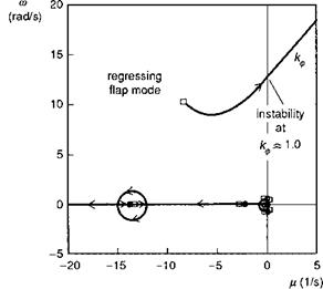
The similar modulus of the roll subsidence and regressing flap modes (both lie roughly on the complex plane circle with radius 10 rad/s), together with the presence of appreciable roll motion in the latter, signals that the use of the 6 DoF weakly coupled approximation for analysing the effects of strong roll control on the stability of lateral motion is unlikely to be valid. Observing the location of the regressing flap mode eigenvalue from Table 5.1, and referring to Fig. 5.2, we can also see that the regressing flap mode lies in the path of the root locus of the strongly controlled roll mode – another clear indication that the situation is bound to change with the addition of higher order flapping dynamics. The root loci of roll attitude feedback to lateral cyclic for the second-order 9 DoF model is shown in Fig. 5.3, revealing that the stability is, as anticipated, changed markedly by the addition of the regressing flap mode. The fuselage eigenvalues no longer coalesce and stiffen the roll axis response into a high – frequency oscillation, but instead the high-gain response energy becomes entrained in a coupled roll/flap mode which becomes unstable at relatively low values of gain, depending on the aircraft configuration. For the Lynx in hover illustrated in Fig. 5.3, the critical value of gain is just below unity. In practice, the response amplitude will be limited by nonlinearities in the actuation system for SCAS operation, or by the pilot reducing his gain and backing out of the control loop. Even for lower values of attitude gain, typical of those found in a SCAS (O(0.2)), the stability of the coupled mode will reduce to levels that could cause concern for flight through turbulence. To alleviate this problem, it is a fairly common practice to introduce notch filters into the SCAS that reduce the feedback signals and response around the frequency of the coupled fuselage/rotor modes. A similar problem arises through the coupling of the roll mode with the regressing lag mode when the roll rate feedback gain is increased, developing into a mode that typically has lower damping than the regressing flap mode;

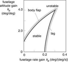
this problem has already been discussed in Chapter 3 (see Section 3.2.1 on lead-lag dynamics) where the work of Curtiss was highlighted (Ref. 5.5). Figure 5.4, taken from Ref. 5.5, shows Curtiss’s estimate of the stability boundary for rate and attitude feedback control. The example helicopter in Ref. 5.5 has an articulated rotor, but the level of attitude gain that drives the fuselage-flap mode unstable is very similar to Lynx, i. e., about 1°/° for zero rate gain. The level of stabilization through rate damping before the fuselage-lag mode is driven unstable is even lower, according to Curtiss, at 0.2°/° s.

High-gain attitude control is therefore seen to present a problem for pilots and SCAS designers. We can obtain some insight into the loss of damping in the roll/flap regressing mode through an approximate stability analysis of the coupled system at the point of instability. We make the assumption that the first-order representation of multi-blade flapping dynamics is adequate for predicting the behaviour of the regressing flap mode. We also neglect the low-modulus fuselage dynamics. From Chapter 3, the equations of motion for the coupled rotor-fuselage angular motion in hover are given by

The hub moment about the aircraft centre of mass is approximated by the expression

Me — ( N. Kp + ГкЛ (5.17)

which includes the moments due to thrust vector tilt and hub stiffness.

Equations 5.11-5.13 represent a fourth-order coupled system and when the atti­tude feedback law, given by eqn 5.10, is included, the order of the system increases to 5. For high values of feedback gain we make the assumption that the coupled roll regressing flap mode and the roll subsidence mode in Fig. 5.3 define the high-modulus system so that no further reduction is possible due to the similar modulus of the eigen­values of these modes. This third-order system has a characteristic equation of the form

A3 + ayU2 + $1^ + ao — 0

The condition for stability of the coupled fuselage-flap mode can be written in the form of a determinant inequality (Ref. 5.6)

(5.19)

After rearrangement of terms and application of reasonably general further approxi­mations, the condition for stability in terms of the roll attitude feedback gain can be written in the form

For the Lynx, the value of attitude gain at the stability boundary is estimated to be approximately 0.8°/° from eqn 5.20. The relatively high value of hub stiffness reduces the allowable level of feedback gain, but conversely, the relatively high rotorspeed on the Lynx serves to increase the usable range of feedback gain. On the Puma, with its slower turning, articulated rotor with higher Lock number, the allowable gain range increases to about 2°/°. Slow, stiff rotors would clearly be the most susceptible to the destabilizing effect of roll attitude to lateral cyclic feedback gain.

Later, in Chapter 6, we shall discuss some of the handling qualities considerations for attitude control. The potential for stability problems in high-gain tracking tasks will be seen to be closely related to the shape of the attitude frequency response at frequencies around the upper end of the range which pilots normally operate in closed-loop tasks. The presence of the rotor and other higher order dynamic elements introduces a lag between the pilot and the aircraft’s response to controls. The pilot introduces an even further delay through neuro-muscular effects and the combination of the two effects reduces the amplitude, and increases the slope of the phase, of the attitude response at high frequency, both of which can lead to a deterioration in the
pilot’s perception of aircraft handling. Further discussion on the influence of SCAS gains on rotor-fuselage stability can be found in Refs 5.7 and 5.8; Ref. 5.9 discusses the same problem through the influence of the pilot modelled as a simple dynamic system.

Now we turn to the second area of application of strong control and stability under constraint, where the pilot or automatic controller is attempting to constrain the flight path, to fly along virtual rails in the sky. We shall see that this is possible only at considerable expense to the stability of the unconstrained modes, dominated in this case by the aircraft attitudes.

Both civil and military helicopters are required to operate in confined spaces, often in conditions of poor visibility and in the presence of disturbed atmospheric conditions. To assist the pilot with flight path (guidance) and attitude (stabilization) control, some helicopters are fitted with automatic stability and control augmentation systems (SCAS) that, through a control law, feedback a combination of errors in aircraft states to the rotor controls. The same effect can be achieved by the pilot, and depending on the level of SCAS sophistication and the task the share of the workload falling on the pilot can vary from low to very high. The combination of aircraft, SCAS and pilot, coupled together into a single dynamic system, can exhibit stability characteristics profoundly different than the natural behaviour discussed in detail in Chapter 4. An obvious aim of the SCAS and the pilot is to improve stability and task performance, and in most situations the control strategy to achieve this is conceptually straightforward – proportional control to cancel primary errors, rate control to quicken the response and integral action to cancel steady-state errors. In some situations, however, the natural control option does not always lead to improved stability and response, e. g., tight control of one constituent motion can drive another unstable. It is of interest to be able to predict such behaviour and to understand the physical mechanisms at work. A potential barrier to physical insight in such situations, however, is the increased dimension of the problem. The sketch of the Lynx SCAS in Chapter 3 (see Fig. 3.36) highlights the complexity of a relatively simple automatic system. Integrating the SCAS with the aircraft will lead to a dynamic system of much higher order than that of the aircraft itself; the pilot behaviour will be even more complex and the scope for deriving further understanding of the dynamic behaviour diminishes, as the complexity and order of the integrated system model increases.

One solution to this dilemma was first discussed by Neumark in Ref. 5.1, who identified that it was possible to imagine control so strong that one or more of the mo­tion variables could actually be held at equilibrium or some other prescribed values. The behaviour of the remaining, unconstrained, variables would then be described by a reduced order dynamical system with dimension even less than the order of the natural aircraft. This concept of constrained flight has considerable appeal for the analysis of motion under strong pilot or SCAS control because of the potential for deriving physical understanding from tractable, low-order analytic solutions. Neumark’s attention was drawn to solving the problem of speed stability for fixed-wing aircraft operating below minimum drag speed; by applying strong control of flight path with elevator, the pilot effectively drives the aircraft into speed instability. In a later report, Pinsker (Ref. 5.2) demonstrated how, through strong control of roll attitude on fixed-wing aircraft with relatively high values of aileron-yaw, a pilot could drive the effective directional stiff­ness negative, leading to nose-slice departure characteristics. Clearly, a helicopter pilot has only four controls to cope with 6 DoFs. If the operational situation demands that the pilot constrains some motions more tightly than others, then there is always a question over the stability of the unconstrained motion. If strong control is required to maintain a level attitude for example, then flight path accuracy may suffer and vice versa. Should strong control of some variables lead to a destabilizing of others, then the pilot should soon recognize this and subsequently share his workload between constraining the primary DoFs and compensating for residual motions of the weakly constrained DoFs. This apparent loss of stability can be described as a pilot-induced oscillation (PIO). However, this form of PIO can be insidious in two respects: first, where the uncon­strained motion departs slowly, making it difficult for the pilot to identify the departure until well developed, and second, where a rapid loss of stability occurs with only a small increase in pilot gain. With helicopters, the relatively loose coupling of the ro­tor and fuselage (compared with the wing and fuselage of a fixed-wing aircraft) can exacerbate the problem of constrained flight to the extent that coupled rotor/fuselage motions can occur which have a limited effect on the aircraft flight path, yet cause significant attitude excursions.

In the following analyses, we shall deal with strong attitude control and strong flight path control separately. We shall make extensive use of the theory of weakly coupled systems (Ref. 5.3), which was used to investigate motion under constraint in Ref. 5.4. The theory is described in Appendix 4A and has already been utilized in Chapter 4 in the derivation of approximations for a helicopter’s natural stability characteristics. The reader is referred to these sections of the book and the references for further elucidation. The method is ideally suited to the analysis of strongly controlled aircraft, when the dynamic motions tend to split into two types – those under control and those not – with the latter tending to form into new modes with stability characteristics quite different from those of the uncontrolled aircraft. In control theory terms, these modes become the zeros of the closed-loop system in the limit of infinite gain.

Everybody’s simulation model is guilty until proved innocent. (Thomas H. Lawrence at the 50th Annual Forum of the AHS, Washington, 1994)

5.1 Introduction and Scope

Continuing the theme of ‘working with models’, this chapter deals with two related topics – stability under constraint and response. The response to controls and atmos­pheric disturbances is the third in the trilogy of helicopter flight mechanics topics; where Chapter 4 focused on trim and natural stability, response analysis is given prime attention in Section 5.3. Understandably, a helicopter’s response characteristics can dominate a pilot’s impression of flying qualities in applied flying tasks or mission task elements. A pilot may, for example, be able to compensate for reduced stability provided the response to controls is immediate and sufficiently large. He may also be quite oblivious to the ‘trim-ability’ of the aircraft when active on the controls. What he will be concerned with is the helicopter’s ability to be flown smoothly, and with agility if required, from place to place, and also the associated flying workload to compensate for cross-couplings, atmospheric disturbances and poor stability. Quantifying the qual­ity of these response characteristics has been the subject of an extensive international research programme, initiated in the early 1980s. Chapter 6 deals with these in detail, but in the present chapter we shall examine the principal aerodynamic and dynamic effects, mostly unique to the helicopter, which lead to the various response characteristics. Response by its very nature is a nonlinear problem, but insight can be gained from investigating small amplitude response through the linearized equations of perturbed motion. This is particularly true for situations where the pilot, human or automatic, is attempting to constrain the motion – to apply strong control – to achieve a task. We discuss this class of problems in Section 5.2, with an emphasis on the kind of changes in the pilot/vehicle stability that can come about, therefore maintaining some continuity with the material in Chapter 4. Section 5.3 follows with an examination of the characteristics of the helicopter’s response to clinical control inputs, and the chapter is concluded with a brief discussion on helicopter response to atmospheric disturbances.

Most of the theory in both Chapters 4 and 5 is concerned with six degree of freedom (DoF) motion, from which considerable insight into helicopter flight dynamics can be gained. However, when the domain of interest on the frequency/amplitude plane includes ‘higher order’ DoFs associated with the rotors, engines, transmission and flight control system, the theory can become severely limited, and recourse to more

complexity is essential. Selected topics that require this greater complexity will be featured in this chapter.

Chapter 3 developed a generalized form for the aerodynamic forces and moments acting on the fuselage; Table 4B.4 presents a set of values of force and moment coefficients, giving one-dimensional, piecewise linear variations with incidence and sideslip. These values have been found to reflect the characteristics of a wide range of fuselage shapes; they are used in Helisim to represent the large angle approximations.

Small angle approximations (-20° < (af, вf) < 20°) for the fuselage aerodynamics of the Lynx, Bo105 and Puma helicopters, based on wind tunnel measurements, are given in eqns 4B.1 – 4B.15. The forces and moments (in N, N/rad, N m, etc.) are given as functions of incidence and sideslip at a speed of 30.48 m/s (100 ft/s). The increased order of the polynomial approximations for the Bo105 and Puma is based on more extensive curve fitting applied to the wind tunnel test data. The small angle approximations should be fared into the large angle piecewise forms.

Lynx

Bo105

Xf loo = -580.6 – 454.0 af + 6.2 a2 + 4648.9 a3 (4B.6)

Yfloo = -6.9 – 2399.0 вf – 1.7 в] + 12.7 в] (4B.7)

Zf100 = -51.1 – 1202.0 af + 1515.7 a2f – 604.2a3 (4B.8)

Mf100 = -1191.8 + 12752.0 af + 8201.3 a2f – 5796.7 a3 (4B.9)

Nf100 = -10028.0 ву (4B.10)

Puma

Xf100 = -822.9 + 44.5 a f + 911.9 a2f + 1663.6 a3 (4B.11)

Yf100 = -11 672.0 в f (4B.12)

Zf100 = -458.2 – 5693.7 af + 2077.3 a2f – 3958.9 af (4B.13)

Mf100 = -1065.7 + 8745.0af + 12473.5af – 10033.0af (4B.14)

Nf100 = -24 269.2 вf + 97 619.0 в} (4B.15)

Empennage aerodynamic characteristics

Following the convention and notation used in Chapter 3, small angle approximations (-20° < (atp, вfn) < 20°) for the vertical tailplane and horizontal fin (normal) aerodynamic force coefficients are given by the following equations. As for the fuselage forces, the Puma approximations have been curve fitted to greater fidelity over the range of small incidence and sideslip angles.

Lynx

Cztp = -3.5 atp (4B.16)

Cyfn = -3.5 вп (4B.17)

Bo105

Cztp = -3.262 atp (4B.18)

Cyfn = -2.704 вп (4B.19)

Puma

Cztp = -3.7 (atp – 3.92ajP) (4B.20)

4B.2 Stability and control derivatives

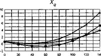
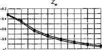
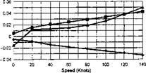
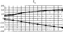
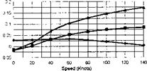
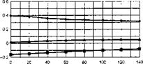
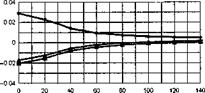
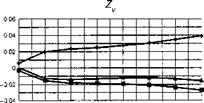
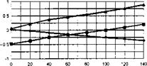
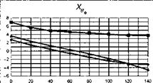
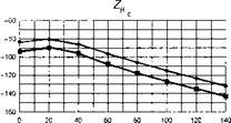
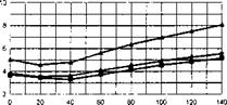
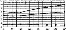
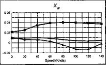
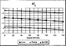
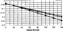
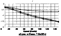
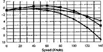
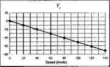
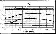
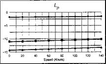
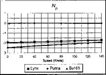
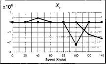
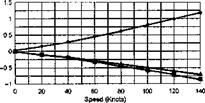
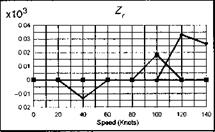
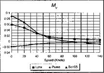
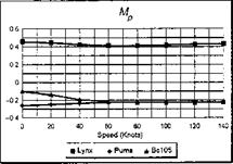
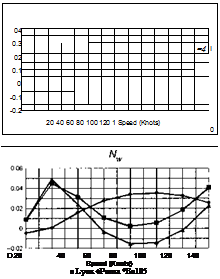
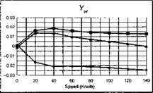
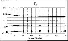
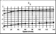
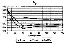
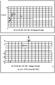
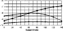
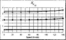
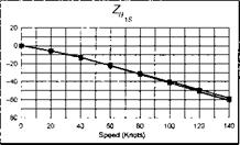
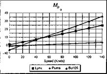
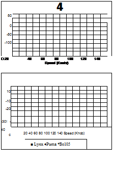
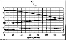
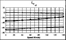
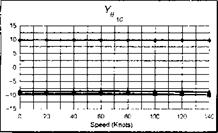
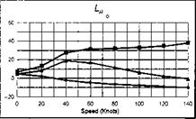
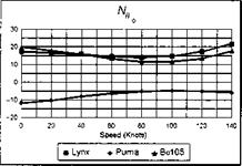
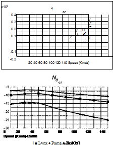
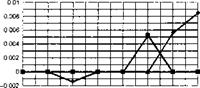
The stability and control derivatives predicted by Helisim for the three subject helicopters are shown in Figs 4B.7-4B.13 as functions of forward speed. The flight conditions correspond to sea level (p = 1.227 kg/m3) with zero sideslip and turn rate, from hover to 140 knots. Figures 4B.7 and 4B.8 show the direct longitudinal and lateral derivatives respectively. Figures 4B.9 and 4B.10 show the lateral to longitudinal, and longitudinal to lateral, coupling derivatives respectively. Figures 4B.11 and 4B.12 illustrate the longitudinal and lateral main rotor control derivatives, and Fig. 4B.13 shows the tail rotor control derivatives. As an aid to interpreting the derivative charts, the following points should be noted:

(1) The force derivatives are normalized by aircraft mass, and the moment derivatives are normalized by the moments of inertia.

(2) For the moment derivatives, pre-multiplication by the inertia matrix has been carried out so that the derivatives shown include the effects of the product of inertia Ixz (see eqns 4.47-4.51).

(3) The derivative units are as follows:

(4) the force/angular velocity derivatives, as shown in the figures, include the trim velocities, e. g.,

7 = 7 U

— Zv q + ‘-d e

*u -0.01 -0.02! -0.03 -0.04 -0.05 -0.06 3 I 0 20 40 60 80 100 120 1 Speed (Knots) 0.05 0 z u ; &V -0.05 -0.1 -0.15 -0.2 г** ~r. у / V -0.25 0 20 40 60 80 100 120 140 Speed (Knots) r 0.12 r M u s. 0.08 0.06 s. 4 0.04* 0.02 N c=. 0 0 20 40 60 80 100 120 140 Speed (Knots) ;*Lynx ♦Puma *Bo105[

Speed (Knots)

60 40 20 -20 20 40 60 80 100 120 140 Speed (Knots)

О 20 40 60 80 100 120 140 Speed (Knots)

[ ■ Lynx ♦ Puma ♦ Bo105 |

0 20 40 60 80 100 120 140 Speed (Knots)

«Lynx ♦Puma -*-Bo105

Speed (Knots)

Speed (Knots)

0 20 40 60 80 100 120 140 Speed (Knots)

x106 M Г 0.8 0.6 0.4 0.2 • у Л / V t r / j V T V . ( -0.2 ( ** 0 20 40 60 80 100 120 1 Speed (Knots) И Lynx *-Puma *Bo105 |

: oo4 : 0 021 і o і : -0.02 Yu -0 04 20 40 60 80 100 120 140 Speed (Knots) Lu ■ X ‘ ‘ ‘ і „ . і 0 —— — 0 20 40 60 80 100 120 140 Speed (Knots)

Speed (Knots) *Lynx – e-Puma *-Bo105

Speed (Knots)

Speed (Knots)

60 40 4 IS ‘ 20 0 c zn 0 20 40 60 60 100 120 1 Speed (Knots) j a Lynx e-Puma *Bo105 |

5 04 % IS -10 c 20 40 60 80 100 120 140 Speed (Knots) | * Lynx ♦Puma *Bo105

x103 0 01 — — <0 C T —– -0 01 -0.02 -0 03 C V ) ■ ■> / ■N I r 20 40 60 80 100 Speed (Knots) 120 140
Speed (Knot3)
Mn
x1Cr
Speed (Knots) ■ Lynx ♦Puma *Bo105
Speed (Knots) I Lynx ♦ Puma * Bo105

Appendix 4C the Trim Orientation Problem

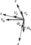
In this section we derive the relationship between the flight trim parameters and the velocities in the fuselage axes system, for use earlier in the chapter. Figure 4C. 1 shows the trim velocity vector Vfe of the aircraft with positive components along the fuselage axes directions x, y and z given by Ue, Ve and We respectively, where subscript e denotes equilibrium.

The trim condition is defined in terms of the trim velocity Vfe, the flight path angle Yfe, the sideslip angle Д. and the angular velocity about the vertical axis Qae. The latter plays no part in the translational velocity derivations. The incidence and sideslip angles are defined as

&e = tan-1 ^ W^ (4C.1)

Pe = sin-1 ((4C.2)

The sequence of discrete orientations required to derive the fuselage velocities in terms of the trim variables is shown below in Fig. 4C.2.

The axes are first rotated about the horizontal y-axis through the flight path angle. Next, the axes are rotated through the track angle, positive to port (corresponding to a positive sideslip angle) giving the orientation of the horizontal velocity component relative to the projected aircraft axes. The final two rotations about the Euler pitch and roll angles bring the axes into alignment with the aircraft axes as defined in Chapter 3, Section 3A.1.

Fig. 4C.1 Flight velocity vector relative to the fuselage axes in trim

The trim velocity components in the fuselage-fixed axis system may then be written as
Ue = Vfe (cos @e cos Yfe cos xe — sin @e sin ye)

(4C.3)

Ve = Vfe (cos Фє cos Yfe sin xe + sin Фє (sin @e cos Yfe cos xe + cos @e sin Yfe))

(4C.4)

We = Vfe (—sin Фє cos Yfe sin xe + cos Фє (sin Qe cos Yfe cos xe + cos @e sin y^

(4C.5)

The track angle is related to the sideslip angle through eqn 4C.4 above. The track angle is then given by the solution of a quadratic, i. e.,

sin

where

and the к coefficients are

Only one of the solutions of eqn 4C.6 will be physically valid in a particular case.

Finally, the relationship between the fuselage angular velocities and the trim vertical rotation rate can be easily derived using the same transformation as for the gravitational forces. Hence,

Pe = -&ae sin Qe (4C.12)

Qe = &ae cos Qe sin Фе (4C.13)

Re = Q, ae cos Qe cos Фє (4C.14)

Note that for conventional level turns, the roll rate p is small and the pitch and yaw rates are the dominant components, with the ratio between the two dependent upon the trim bank angle. In trim at high climb or descent rates the pitch angle can be significantly different from zero, increasing the roll rate in the turn manoeuvre.

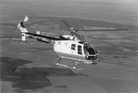
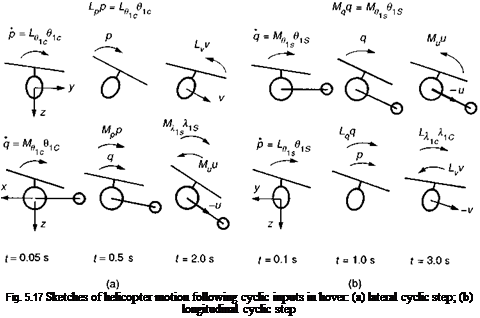
The German DLR variable stability (fly-by-wire/light) Bo105 S3
(Photograph courtesy of DLR Braunschweig)