Our heavyweight helicopter equal in the world does not have
In Rostov started production of the most load-lifting rotary-wing car The Russian holding «Helicopt[...]

Everything about aircrafts and helicopters. News and events in aviation worldwide. Civil, transportation, military helicopters and airplanes.

Everything about aircrafts and helicopters. News and events in aviation worldwide. Civil, transportation, military helicopters and airplanes.

Everything about aircrafts and helicopters. News and events in aviation worldwide. Civil, transportation, military helicopters and airplanes.

Everything about aircrafts and helicopters. News and events in aviation worldwide. Civil, transportation, military helicopters and airplanes.


Experience has shown that a large percentage, perhaps as much as 65%, of the life-cycle cost of an aircraft is committed during the early design and definition phases of a new development program. It is clear, furthermore, that the handling qualities of military helicopters are also largely committed in these early definition phases and, with them, much of the mission capability of the vehicle. For these reasons, sound design standards are of paramount importance both in achieving desired performance and avoiding unnecessary program cost. ADS-33 provides this sound guidance in areas of flying qualities, and the authority of the new standards is anchored in a unique base ofadvanced simulation studies and in-flight validation studies, developed under the TTCP collaboration.
(From the TTCP* Achievement Award, Handling Qualities Requirements for Military Rotorcraft, 1994)
6.1 General Introduction to Flying Qualities
In Chapter 2, the Introductory Tour of this book, we described an incident that occurred in the early days of helicopter flying qualities testing at the Royal Aircraft Establishment (Ref. 6.1). An S-51 helicopter was being flown to determine the longitudinal stability and control characteristics, when the pilot lost control of the aircraft. The aircraft continued to fly in a series of gross manoeuvres before it self-righted and the pilot was able to regain control and land safely. The incident highlighted the potential consequences of poor handling qualities – pilot disorientation and structural damage. In the case described the crew were fortunate; in many other circumstances these consequences can lead to a crash and loss of life. Good flying qualities play a major role in contributing to flight safety. But flying qualities also need to enhance performance, and this tension between improving safety and performance in concert is ever present in the work of the flying qualities engineer. An arguable generalization is that military requirements lean towards an emphasis on performance while civil requirements are more safety oriented. We shall address this tension with some fresh insight later in this chapter, but first we need to bring out the scope of the topic.
The ‘original’ definition of handling qualities by Cooper and Harper (Ref. 6.2),
Those qualities or characteristics of an aircraft that govern the ease and precision with which a pilot is able to perform the tasks required in support of an aircraft role
|
still holds good today, but needs to be elaborated to reveal the scope of present day and future usage. Figure 6.1 attempts to do this by illustrating the range of influences – those external to and those internal to the aircraft andpilot. This allows us to highlight flying qualities as the synergy between these two groups of influencing factors. To emphasize this point, it could be argued that without a complete description of the influencing factors, it is ambiguous to talk about flying qualities. It could also be argued that there is no such thing as a Level 1 or a Level 2 aircraft, in the Cooper-Harper parlance. The quality can be referenced only to a particular mission (or even mission task element (MTE)) in particular visual cues, etc. In a pedantic sense this argument is hard to counter, but we take a more liberal approach in this book by examining each facet, each influencing factor, separately, and by discussing relevant quality criteria as a sequence of one-dimensional perspectives. We shall return to the discussion again in Chapter 7.
In the preceding paragraph, the terms handling qualities and flying qualities have deliberately been used interchangeably and this flexibility is generally adopted throughout the book. At the risk of distracting the reader, it is fair to say, however, that there is far from universal agreement on this issue. In an attempt to clarify and emphasize the task dependencies, Key, as discussed in Ref. 6.4, proposes a distinction whereby flying qualities are defined as the aircraft’s stability and control characteristics (i. e., the internal attributes), while handling qualities are defined with the task and environment included (external influences). While it is tempting to align with this perspective, the author resists on the basis that provided the important influence of task and environment are recognized, there seems no good reason to relegate flying to be a subset of handling.
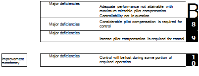
In the structure of current Civil and Military Requirements, good flying qualities are conferred to ensure that safe flight is guaranteed throughout the operational flight envelope (OFE). The concept of flying quality requires a measurement scale to judge an aircraft’s suitability for role, and most of the efforts of flying qualities engineers over the years have been directed at the development of appropriate scales and metrics, underpinned and substantiated by flight test data. The most developed and widely recognized quality scale is that due to Cooper and Harper (Ref. 6.2). Goodness, or quality, according to Cooper-Harper, can be measured on a scale spanning three levels (Fig. 6.2). Aircraft are normally required to be Level 1 throughout the OFE (Refs 6.5, 6.6); Level 2 is acceptable in failed and emergency situations but Level 3 is considered unacceptable. The achievement of Level 1 quality signifies that a minimum required standard has been met or exceeded in design, and can be
 |
|||
|
|||
|
|||
|
|
||
 |
|||
![]()
expected to be achieved regularly in operational use, measured in terms of task performance and pilot workload. Compliance flight testing is required to demonstrate that a helicopter meets the required standard and involves clinical measurements of flying qualities parameters for which good values are known from experience. It also involves the performance of pilot-in-the-loop MTEs, along with the acquisition of subjective comments and pilot ratings. The emphasis on minimum requirements is important and is made to ensure that manufacturers are not unduly constrained when conducting their design trade studies. Establishing the quality of flying, therefore, requires objective and subjective assessments which are the principal topics of Chapters 6 and 7 respectively.
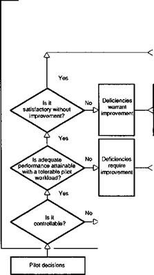
We refer to the subjective pilot ratings given on the Cooper-Harper scale as handling qualities ratings (HQRs). HQRs are awarded by pilots for an aircraft flying an MTE, and are determined by the pilot following through the decision tree shown in Fig. 6.2, to arrive at his or her rating based on their judgement of task performance achieved and pilot workload expended. The task performance requirements will have been set at desired and adequate levels and the pilot should have sufficient task cues to support the judgement of how well he or she has done. In a well-defined experiment this will usually be the case, but poorly defined flight tests can lead to increased scatter between pilots on account of the variations in perceived performance (see Chapter 7 for more discussion on this topic). Task performance can be measured, be it flight path accuracy, tracking performance or landing scatter and the results plotted to give a picture of the relative values of flying quality. The other side of the coin, pilot workload, is much more difficult to quantify, but we ask test pilots to describe their workload in terms of the compensation they are required to apply, with qualifiers – minimal, moderate, considerable, extensive and maximum. The scale implies an attempt to determine how much spare capacity the pilot has to accomplish other mission duties or to think ahead and react quickly in emergencies. The dual concepts of ‘attentional demand’ and ‘excess control capacity’ have been introduced by McRuer (Ref. 6.7) to distinguish and measure the contributing factors to the pilot workload. However subjective, and hence flawed by the variability of pilot training and skill, the use of HQRs may seem, along with supporting pilot comment and task performance results, it has dominated flying qualities research since the 1960s. It is recognized that at least three pilots should participate in a flying qualities experiment (preferably more, ideally five or six) and that HQRs can be plotted with mean, max and min shown; a range of more than two or three pilot ratings should alert the flying qualities engineer to a fault in experimental design. These are detailed issues and will be addressed later in Chapter 7, but the reader should register the implied caution; misuse of HQRs and the Cooper-Harper scale is all too easy and too commonly found.
Task performance requirements drive HQRs and give modern military flying qualities standards, like the US Army’s ADS-33C (Ref. 6.5), a mission orientation. The flying qualities are intended to support the task. In a hierarchical manner, ADS-33C defines the response types (i. e., the short-term character of response to control input) required to achieve Level 1 or 2 handling qualities for a wide variety of different MTEs, in different usable cue environments (UCE) for normal and failed states, with full and divided pilot attention. Criteria are defined for both hover/low speed and forward flight, in recognition of the different MTEs and related pilot control strategies in the two operating regimes. Within these flight phases, the criteria can be further related to the level of aggressiveness used by the pilot in attacking a manoeuvre or MTE. At a deeper level, the response characteristics are broken down in terms of amplitude and frequency range, from the small amplitude, higher frequency requirements set by criteria like equivalent low-order system response or bandwidth, to the large amplitude manoeuvre requirements set by control power. By comparison, the equivalent fixed – wing requirements, MIL-F-8785C (Ref. 6.6), take a somewhat different perspective, with flight phases and aircraft categories, but the basic message is the same – how to establish flying quality in mission-related tasks. The innovations of ADS-33 are many and varied and will be covered in this chapter; one of the many significant departures from its predecessor, MIL-H-8501A, is that there is no categorization according to aircraft size or, explicitly, according to role, but only by the required MTEs. This emphasizes the multi-role nature of helicopters and gives the new specification document generic value. Without doubt, ADS-33 has resulted in a significant increase in attention to flying qualities in the procurement process and manufacturing since its first publication in the mid-1980s, and will possibly be perceived in later years as marking a watershed in helicopter development. The new flying qualities methodology is best illustrated by Key’s diagram (Ref. 6.8) shown in Fig. 6.3.
In this figure the role of the manufacturer is highlighted, and several of the ADS – 33 innovations that will be discussed in more detail later in this chapter are brought out, e. g., response types and the UCE.
|
Fig. 6.3 Conceptual framework for handling qualities specification (Ref. 6.8) |
In a similar timeframe to the development of ADS-33C, the revision to the UK’s Def Stan 00970 was undertaken (Ref. 6.9). This document maintained the UK tradition of stating mandatory requirements in qualitative terms only, backed up with advisory leaflets to provide guidance on how the characteristics may be achieved. An example of the 970 requirements, relating to response to control inputs, reads
The third aspect in this section is concerned with the sensitivity of aircraft, crew, weapon system, passengers or equipment to atmospheric disturbances, taken together under the general heading – ride qualities. Reference 5.57 discusses the parameters used to quantify ride bumpiness for military fixed-wing aircraft, in terms of the normal acceleration response. For helicopter applications, the meaning of ride qualities, in terms of which flight parameters are important, is a powerful function of the aircraft role and flight condition. For example, the design of a civil transport helicopter required to cruise at 160 knots may well consider the critical case as the number of, say, 1/2 g vertical bumps per minute in the passenger cabin when flying through severe turbulence. For an attack helicopter the critical case may be the attitude perturbations in the hover, while cargo helicopters operating at low speed with underslung loads may have flight path displacement as the design case. For the first example quoted, a direct parallel can be drawn from fixed-wing experience. In Ref. 5.57 Jones promotes the application of the SDG method to aircraft ride qualities in the following way. We have already introduced the concept of the tuned gust, producing the maximum or tuned transient response. Based on tuned gust analysis, the predicted rate of occurrence of vertical bumps can be written in the form
where
ny is the average number of aircraft normal acceleration peaks with magnitude greater than y, per unit distance flown;
a and в reflect statistical properties of the patch of turbulence through which the aircraft is flying;
H is the tuned gust scale (length);
Y is the tuned response (Fig. 5.35(c)); к is the gust length sensitivity.
In addition to its relative simplicity, this kind of formulation has the advantage that it caters for structured turbulence and hence structured aircraft response. The approach can be extended to cases where the gust field is better represented by gust pairs and other more complicated patterns, with associated complex tuning functions. The basis of the SDG method is the assumption that structured atmospheric disturbance is more correctly and more efficiently modelled by localized transient features. The wavelet
|
Fig. 5.36 Transient response quickness as a ride qualities parameter: (a) quickness extraction; (b) quickness chart |
analysis has provided a sound theoretical framework for extending the forms of transient disturbance and response shape to more deterministic analyses. At the same time, new handling qualities criteria are being developed that characterize the response in moderate amplitude manoeuvres, also in terms of transient response. The so-called attitude ‘quickness’ (Ref. 5.58), to be discussed in more detail in Chapter 6, represents a transient property of an aircraft’s response to pilot control inputs. The same concept can be extended to the analysis of the aircraft response to discrete gusts, as summarized in Fig. 5.36. The response quickness, shown in Fig. 5.36(a) applied to the normal velocity response, is extracted from a signal by identifying significant changes (Aw – strictly the integral of acceleration) and estimating the associated maximum or peak rate of change, in this case peak normal acceleration (aZpk); the quickness associated with the event is then given by the discrete parameter
az,
Qw = (5.84)
Aw
Clearly, each discrete gust has an associated quickness, which actually approximates to 1/L in the limit of a linear ramp gust. Quickness values can then be plotted as points on charts as shown in Fig. 5.36(b). In this case we have plotted the values as a function of the gust input intensity, assuming a unique relationship between the input-output pair. Bradley et al. (Ref. 5.44) have shown that the quickness points group along the tuning lines, related to у, as shown in hypothetical form in Fig. 5.36(b). Also shown in the figure are contours of equi-responsiveness or equi-comfort which suggest a possible format for specifying ride quality.
The ongoing research on the topic of ride qualities is likely to produce alternative approaches to modelling and analysing disturbance and response, derived as ever from different perspectives and experiences. The key to more general acceptance will certainly be validation with real-world experience and test data, and it is in this area that the major gaps lie and much more work needs to be done. There are very few sets of test data available, and perhaps none that is fully documented, that characterize the disturbance and the helicopter response to turbulence in low-level nap-of-the-earth flight; it is a prime area for future research. Data are important to validate simulation modelling and also to establish new ride criteria that can be used with confidence in the design of new aircraft and the associated automatic flight control systems. The current specification standards for rotorcraft handling do not make any significant distinction between the performance associated with the response to controls and disturbances. Clearly, an aircraft which is naturally agile is also likely to be naturally bumpy, and an active control system will need to have design features that cope with both handling and ride quality requirements. Fortunately, the handling qualities standards, perhaps the more important of the two, are now, in general, better understood, having been the subject of intense investigations over the last 15 years. Handling qualities forms the subject of the remaining two chapters of this book.
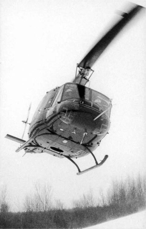
The Canadian NRC variable stability (fly-by-wire) Bell 205 during
a handling qualities evaluation near Ottawa
(Photograph from the author’s collection)
Consideration of the response of helicopters to atmospheric disturbances needs to take account of a number of factors. We have seen from the simple Level 1 modelling described in Chapter 3 that the rotor response to in-plane and out-of-plane velocity perturbations is distributed over the frequencies associated with the harmonics of rotorspeed. In high-speed flight the force response at the rotor hub tends to be dominated by the n-per-rev and 2n-per-rev components, and many studies have focused on important fatigue and hub vibratory loading problems (e. g., Refs 5.52, 5.53). Only the zero harmonic forces and the first harmonic moments lead to zero-frequency hub and fuselage response and thus affect the piloting task directly. Several studies (e. g., Refs 5.38-5.40) have concentrated on investigating factors that alleviate the fuselage response relative to the sharp bump predicted by ‘instantaneous’ models, typified, for example, by eqn 5.77. Rotor-fuselage penetration effects coupled with any gust ramp characteristics tend to dominate the alleviation with secondary effects due to rotor dynamics and blade elasticity. Rotor unsteady aerodynamics can also have a significant influence on helicopter response, particularly the inflow/wake dynamics (see Chapter 3). An important aspect covered in several published works concerns the cyclo-stationary nature of the rotor blade response (Refs 5.42, 5.43, 5.54, 5.55). Essentially, the radial distribution of turbulence effects varies periodically and the gust velocity environments at the rotor hub and rotor blade tip are therefore substantially different. If a helicopter is flying through a sinusoidal vertical gust field with scale L and intensity Wgm, then the turbulence velocities experienced at the rotor hub and blade tip are given by the expressions
wgh)(t) = wgm sin j (5.81)
(t) 12n Vt 2n R }
wgt) = wgm sin j —————- — cos (5.82)
where Vis the combined forward velocity of the aircraft and gust field. Response studies that include only hub-fixed turbulence models (eqn 5.81) and assume total immersion of the rotor at any instant clearly ignore much of the local detail in the way the individual blades experience the gust field. At low speed with scales O(R), this approximation becomes invalid, and recourse to more detailed modelling is required. Assuming the gust field varies linearly across the rotor allows the disturbance to be incorporated as an effective pitch (roll) rate or non-uniform inflow component. This level of approximation can be regarded as providing an interim level of accuracy for gust scales that are larger than the rotor but that still vary significantly across the disc at any given time. In Ref. 5.56, a study is reported on the validity of various approximations to the way in which rotor blades respond to turbulence, suitable for incorporation into a real-time simulation model. The study concluded that the modelling of two-dimensional turbulence effects is likely to be required, and that approximating the turbulence intensity over a whole blade by the value at the 3/4 radius would provide adequate levels of accuracy.
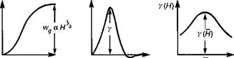
In addition to characterizing the atmospheric disturbance, the SDG approach, augmented with the transient wavelet analysis, provides a useful insight into helicopter response. The concept of the tuned response is illustrated in Fig. 5.35. Associated with each ramp gust input (Fig. 5.35(a)) we assume the response variable of interest has a single dominant peak, of amplitude у, as shown in Fig. 5.35(b). If the helicopter model is excited with each member of the family of equi-probable gusts, according to the von Karman PSD, then we find, in general, that the response peak function takes the form given in Fig. 5.35(c). There exists a tuned gust length H that produces a ‘resonant’ response from the helicopter. This transient response resonance is the equivalent of the resonance frequency in the frequency domain representation, and can be used to quantify a helicopter’s ride qualities.
H-
![]()
![]()

 (a)
(a)
In the UK Airworthiness Defence Standard (Ref. 5.45), turbulence intensity is characterized by four bands: light (0-3 ft/s), moderate (3-6 ft/s), severe (6-12 ft/s) and extreme (12-24 ft/s). A statistical approach to turbulence refers to the probability of equalling or exceeding given intensities at defined heights above different kinds of terrain. A second important property of turbulence is the relationship between the intensity and the spatial or temporal scale or duration, which also varies with height above terrain. Such a classification has obvious attractions for design and certification purposes, and the extensions of fixed-wing methods to helicopters are generally applicable at operating heights above about 200 ft. Below this height, the dearth of measurements of three-dimensional atmospheric disturbances means that the characterization of turbulence is less well understood, with the distinct exception of airflow around man-made constructions (Ref. 5.46). For the purposes of this discussion, we circumvent this dearth of knowledge and concern ourselves only with the general modelling issues rather than specific cases, but it is important to note that extensions of results from fixed-wing studies may well not apply to helicopters. Another area where this read-across has to be reinterpreted is the treatment of turbulence scale length. In fixed-wing work a common approximation assumes a ‘frozen-field’ of disturbances, such that the scale length and duration are related directly through the forward speed of the aircraft. For helicopters in hover or flying through winds at low speed, this approach is clearly not valid and it is more appropriate to consider the aircraft flying through (or hovering in) a steady wind with the turbulence superimposed.
The most common form of turbulence model involves the decomposition of the velocity into frequency components, where the rms of the aircraft response can be related to the rms intensity of the turbulence. In Ref. 5.45, this power spectral density (PSD) method is recommended for investigations of general handling qualities in continuous turbulence. The PSD contains information about the excitation energy within the atmosphere as a function of frequency (or spatial wavelength), and several models exist based on measurements of real turbulence. For example, the von Karman PSD of the vertical component of turbulence takes the form (Refs 5.47, 5.48)
where the wavenumber v = frequency/airspeed, L is the turbulence scale and a is the rms of the intensity. The von Karman method assumes that the disturbance has Gaussian properties and the extensive theory of stationary random processes can be brought to bear when considering the response of an aircraft as a linear system. This is clearly a strength of the approach but it also reveals a weakness. A significant shortcoming of the basic PSD approach is its inability to model any detailed structure in the disturbance. Large peaks and intermittent features are smoothed over as the amplitude and phase characteristics are assumed to be uniformly distributed across the spectrum. Any phase correlations in the turbulence record are lost in the PSD process, hence removing the capability of sinusoidal components reinforcing one another. Atmospheric disturbances with highly structured character, corresponding for example to shear layers exhibiting sharp velocity gradients, are clearly important for helicopter applications in the wake of hills and structures, and a different form of modelling is required in these cases.
|
Fig. 5.33 Elemental ramp gust used in the statistical discrete gust approach |
The statistical discrete gust (SDG) approach to turbulence modelling was developed by Jones at DRA (RAE) for fixed-wing applications (Refs 5.49-5.51), essentially to cater for more structured disturbances, and appears to be ideally suited for low – level helicopter applications. In Ref. 5.45, the SDG method is recommended for the assessment of helicopter response to, and recovery from, large disturbances. The basis of the SDG approach is an elemental ramp gust (Fig. 5.33) with gradient distance (scale) H and gust amplitude (intensity) Wg. A non-Gaussian turbulence record can be reconstituted as an aggregate of discrete gusts of different shapes and sizes; different elemental shapes, with self-similar characteristics (Ref. 5.49), can be used for different forms of turbulence. One of the properties of turbulence, correctly modelled by the PSD approach, and that the SDG method must preserve, is the shape of the PSD itself which appears to fit measured data well. This so-called energy constraint (Ref. 5.50) is satisfied by the self-similar relationship between the gust amplitude and length in the aggregate used to build the equivalent SDG model. For example, with the VK spectrum, the relationship takes the form wg a H1/3 for gusts with length small compared with the reference spectral scale L.
Where the PSD approach adopts frequency-domain, linear analysis, the SDG approach is essentially a time-domain, nonlinear technique. Since the early development of the SDG method, a theory of general transient signal analysis has been developed, providing a rational framework for its use. The basis of this analysis is the so-called ‘Wavelet’ transform, akin to the Fourier transform, but returning a new time-domain function of scale and intensity (Ref. 5.51). The SDG elements can now be interpreted as a particular class of wavelet, and a turbulence time history can be decomposed into a combination of wavelets adopting the so-called adaptive wavelet analysis (Ref. 5.48). These new techniques provide considerably more flexibility in the modelling of structured turbulence and should find regular use in helicopter response analysis.
To close this brief review of turbulence modelling, Fig. 5.34 illustrates the comparison between two forms of turbulence record reconstruction (Ref. 5.48). The measurements exhibit features common to real atmospheric disturbances – sharp velocity gradients associated with shear layers and periods of relative quiescence (Fig. 5.34(a)). Figure 5.34(b) shows the turbulence reconstructed using measured amplitude components with random phase components from the PSD model. From a PSD perspective, the information in Fig. 5.34(b) is identical to the measurements, but it can be seen that all structured features in the measurements have apparently disappeared in the
|
Fig. 5.34 Influence of Fourier amplitude and phase on the structure of atmospheric turbulence: (a) measured atmospheric turbulence; (b) reconstruction using measured amplitude components; (c) reconstruction using measured phase components |
reconstruction process. Figure 5.34(c), on the other hand, has been reconstructed using the measured phase components with random amplitude components from the PSD model. The structure has been preserved in this process, clear evidence of the nonGaussian characteristics of these turbulence measurements, where the real phase correlation has preserved the reinforcement of energy present in the concentrated events. These structured features of turbulence are important for helicopter work. They occur in the nap-of-the-earth and close to oil rigs and ships. Their scales can also be quite small and, at low helicopter speeds, scale lengths as small as the rotor radius can influence ride and handling.
Helicopter flying qualities criteria try to take account of the influence of atmospheric disturbances on the response of the aircraft in terms of required control margins close to the edge of the operational flight envelope and the consequent pilot fatigue caused by the increased workload. We can obtain a coarse understanding of the effects of gusts on helicopter response through linear analysis in terms of the aerodynamic derivatives. In Chapter 2 we gave a brief discourse on response to vertical gusts, which we can recall here to introduce the subject. Assuming a first-order initial heave response to vertical gusts, we can write the equation of motion in the form of eqn 5.76:
■ Zww ^ Zwwg (5.76)
dt
The heave damping derivative Zw now defines both the transient response and the gust input gain. The initial normal acceleration in response to a sharp edge gust is given by the expression
In Chapter 2, and later in Chapter 4, we derived approximate expressions for the magnitude of the derivative Zw, and hence the initial heave bump, for hover and forward flight in the forms
Hover:
Forward flight:
A key parameter in the above expressions is the blade loading (Ma/Ab), to which the gust response is inversely proportional. The much higher blade loadings on rotorcraft, compared with wing loadings on fixed-wing aircraft, are by far the single most significant reason why helicopters are less sensitive to gusts than are the corresponding fixed-wing aircraft of the same weight and size. An important feature of helicopter gust response in hover, according to eqn 5.78, is the alleviation due to the build-up of rotor inflow. However, as we have already seen in Section 5.3.2, rotor inflow has a time constant of about 0.1 s, hence the alleviation will not be as significant in practice. In forward flight the gust sensitivity is relatively constant above speeds of about 120 knots. This saturation effect is due to the cyclic blade loadings; the loadings proportional to forward speed are dominated by the one-per-rev lift. A similar analysis can be conducted for the response of the helicopter in surge and sway with velocity perturbations in three directions. This approach assumes that the whole helicopter is immersed in the gust field instantaneously, thus ignoring any penetration effects or the cyclic nature of the disturbance caused by the rotating blades. An approximation to the effects of spatial variations in the gust strength can also be included in the form of linear variations across the scale of the fuselage and rotor through effective rate derivatives (e. g., Mq, Lp, Nr). In adopting this approach care must be taken to include only the aerodynamic components of these derivatives to derive the gust gains.
While the 6 DoF derivatives provide a useful starting point for understanding helicopter gust response, the modelling problem is considerably more complex. Early work on the analysis of helicopter gust response in the 1960s and 1970s (Refs 5.365.41) examined the various alleviation factors due to rotor dynamics and penetration effects, drawing essentially on analysis tools developed for fixed-wing applications. More recently (late 1980s and 1990s) attention has been paid to understanding response with turbulence models more representative of helicopter operating environments, e. g., nap of the earth and recovery to ships (Refs 5.42, 5.43). These two periods of activity are not obviously linked and the underlying subject of ride qualities has received much less attention than handling qualities in recent years; as such there has not been a coherent development of the subject of helicopter (whole-body) response to gusts and turbulence. What can be said is that the subject is considerably more complex than the response to pilot’s controls and requires a different analytical framework for describing and solving the problems. The approach we take in this section is to divide the response problem into three parts and to present an overview: first, the characterization and modelling of atmospheric disturbances for helicopter applications; second, the modelling of helicopter response; third, the derivation of suitable ride qualities. A flavour running through this overview will be taken from current UK research to develop a unified analytic framework for describing and solving the problems contained in all three elements (Ref. 5.44).
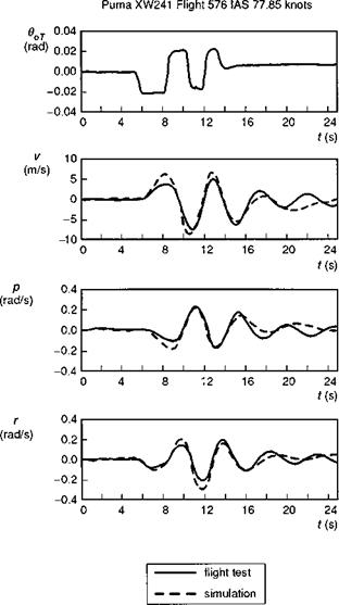
In this section we examine the characteristics of the coupled yaw/roll response to pedal control inputs in forward flight; attention will be focused on comparison with test data from the DRA Puma helicopter. Yaw/roll motions are coupled through a variety of different physical mechanisms. Even at the hover, any vertical offset of the tail rotor from the aircraft centre of gravity will give rise to a rolling moment from tail rotor collective. As forward speed increases, the forces and moments reflected in the various coupled stability derivatives, e. g., dihedral Lv, adverse yaw Np, combine to form the character of the Dutch roll mode discussed in Chapter 4. Figure 5.28, taken from Ref. 5.33, illustrates the comparison of yaw, roll and sideslip responses from flight and Helisim following a 3211 multi-step pedal control input. It can be seen that the simulation overpredicts the initial response in all 3 DoFs and also appears to overpredict the damping and period of the free oscillation in the longer term. In Chapter 4 we examined approximations to this mode, concluding that for both the Puma and Bo105, a 3 DoF yaw/roll/sideslip model was necessary but that, provided the sideways motion was small compared with sideslip, a second-order approximation was adequate; with this approximation, the stability is then characterized by the roots of the
(5.72)
If the ‘true’ values of the stability and control derivatives were known, then this kind of approximation may be able to help to explain where the modelling deficiencies lie. Estimates of the Puma derivatives derived by the DLR using the test data in Fig. 5.28 are shown in Table 5.4, along with Dutch roll eigenvalues for three different cases – the fully coupled 6 DoF motion, lateral subset and the approximation given by eqn 5.69. It can be seen that the latter accounts for about 80% of the damping and more than 90% of the frequency for the flight results (compare Л(1) with Л(3)) and therefore serves as a representative model of Dutch roll motion; note that theory overpredicts the damping by more than 60% and underpredicts the frequency by 20%.
|
Fig. 5.28 Response to pedal 3211 input – comparison of flight and simulation for Puma at 80 knots (Ref. 5.33) |
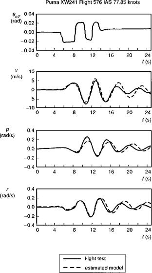
Figure 5.29 shows a comparison between flight measurements and the 3 DoF second-order approximation using the flight-estimated derivatives in Table 5.4. The comparison is noticeably better in the short term, but the damping appears now to be slightly underpredicted, consistent with the comparison already noted between Л(1) with Л(3). Looking more closely at the derivatives in Table 5.4, we see that the most striking mismatch between flight and theory is the overprediction of the yaw damping and control sensitivity by about 70% and the underprediction of the roll damping and dihedral effects by 30 and 20%, respectively. The Helisim prediction of adverse yaw
|
Derivative |
Flight test – DLR |
Helisim |
|
Yv |
-0.135 (0.0019) |
-0.125 |
|
Lv |
-0.066 (0.0012) |
-0.055 |
|
Nv |
0.027 (0.0002) |
0.0216 |
|
Lp |
-2.527 (0.0534) |
-1.677 |
|
Np |
-0.395 (0.0092) |
-0.174 |
|
Lr |
-0.259 (0.0343) |
0.142 |
|
Nr |
-0.362 (0.0065) |
-0.57 |
|
Llat |
-0.051 (0.0012) |
-0.043 |
|
Nlat |
-0.008 (0.0002) |
-0.0047 |
|
Lped |
0.011 (0.0007) |
0.0109 |
|
Nped |
-0.022 (0.0001) |
-0.0436 |
|
Tlat |
0.125 |
0.0 |
|
A(1) |
-0.104 ± 1.37i |
-0.163 ± 1.017i |
|
a(2) |
-0.089 ± 1.27i |
-0.166 ± 1.08i |
|
2£^ |
0.1674 |
0.390 |
|
ОУ2 |
1.842 |
1.417 |
|
A(3) |
-0.081 ± 1.34i |
-0.199 ± 1.199i |
|
Table 5.4 Dutch roll oscillation characteristics |
|
A(1) Dutch roll (fully coupled). A(2) Dutch roll (lateral subset). A(3) Dutch roll (second-order roll/yaw/sideslip) approximation. Numbers in parentheses give the standard deviation of the estimated derivatives. |
Np is less than half the value estimated from the flight data. A simple adjustment to the yaw and roll moments of inertia, albeit by a significant amount, would bring the theoretical predictions of damping and control sensitivity much closer to the flight estimates. Similarly, the product of inertia Ixz has a direct effect on the adverse yaw. Moments of inertia are notoriously difficult to estimate and even more difficult to measure (particularly roll and yaw), and errors in the values used in the simulation model of as much as 30% are possible. However, the larger discrepancies in the yaw axis are unlikely to be due solely to incorrect configuration data. The absence of any interactional aerodynamics between the main rotor wake/fuselage/empennage and tail rotor is likely to be the cause of some of the model deficiency. Typical effects unmodelled in the Level 1 standard described in Chapter 3 include reductions in the dynamic pressure in the rotor/fuselage wake at the empennage/tail rotor and sidewash effects giving rise to effective v acceleration derivatives (akin to Mw from the horizontal tailplane).
The approximation for the Dutch roll damping given by eqn 5.70 can be further reduced to expose effective damping derivatives in yaw and sideslip:
In both cases the additional effect due to rolling motion is destabilizing, with the adverse yaw effect reducing the effective yaw damping by half. The adverse yaw is almost entirely a result of the high value of the product of inertia Ixz, coupling the
|
Fig. 5.29 Response to pedal 3211 input – comparison of flight and identified model – Puma at 80 knots (Ref. 5.33) |
roll damping into the yaw motion. The damping decrements due to rolling manifest themselves as a moment (eqn 5.73) and a force (eqn 5.74) reinforcing the motion at the effective centre of the oscillation. This interpretation is possible because of the closely coupled nature of the motion. The yaw, roll and sideslip motions are locked in a tight phase relationship in the Puma Dutch roll – sideslip leading yaw rate by 90° and roll rate lagging behind yaw rate by 180°. Hence, as the aircraft nose swings to starboard with a positive yaw rate, the aircraft is also rolling to port (induced by the dihedral effect from the positive sideslip) thus generating an adverse yaw Np in the same direction as the yaw rate.
 |
||
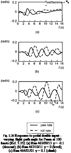
The powerful effect of the damping decrement from adverse yaw can be even more vividly illustrated with an example taken from Refs 5.34 and 5.35. Figure 5.30 presents a selection of Puma flight results comparing the roll and yaw response in the Dutch roll mode at 100 knots in descending, level and climbing flight; the control input is a pedal doublet in all three cases. It can be seen that the stability of the oscillation is affected dramatically by the flight path angle. In descent, the motion has virtually decayed after about 10 s. In the same time frame in climbing flight, the pilot is about to intervene to inhibit an apparently violent departure. A noticeable feature of the response in the three conditions is the changing ratio of roll to yaw. Reference 5.35 discusses this issue and points out that when the roll and yaw motions are approximately 180° out of phase, the effective damping can be written in the form
|
|
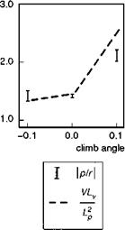
Fig. 5.31 Variation of Dutch roll oscillation roll/yaw ratio with flight path angle (Ref. 5.35)
Figure 5.31 compares the variation of the ratio p/r in the three conditions with the approximation in eqn 5.73 (V Lv/Lp), providing additional validation of this relatively simple approximation for a complex mode. The ratio of roll to yaw motion in the Dutch roll mode was discussed at the end of Chapter 4 in the context of the SA330 Puma. There it was shown how small perturbation linear analysis predicted Dutch roll instability at about 120 knots. When larger sideslip perturbations were used to calculate the derivatives however, the nonlinearity in the yawing moment with sideslip led to a much larger value for the weathercock stability and a stable Dutch roll (see Fig. 4.28). This strong nonlinearity leads to the development of a limit cycle in the Puma at high speed. Figure 5.32 compares the Puma Dutch roll response for the small perturbation linear Helisim with the full nonlinear Helisim, following a 5 m/s initial disturbance in sideslip from a trim condition of 140 knots. The linear model predicts a rapidly growing unstable motion with roll rates of more than 70°/s developing after only three oscillation cycles. The nonlinear response, which is representative of flight behaviour, indicates a limit cycle with the oscillation sustained at roll and yaw rate levels of about 5°/s and 10°/s, respectively; the sideslip excursions are about 10°, a result consistent with the stability change in Fig. 4.28 lying between sideslip perturbations of 5° and 15°.
The Dutch roll is often described as a ‘nuisance’ mode, in that its presence confers nothing useful to the response to pedal or lateral cyclic controls. The Dutch roll mode also tends to become rather easily excited by main rotor collective and longitudinal cyclic control inputs, on account of the rotor/engine torque reactions on the fuselage. In Chapter 6, criteria for the requirements on Dutch roll damping and frequency are presented and it is apparent that most helicopters naturally lie in the unsatisfactory area, largely due to the relatively high value for the ratio of dihedral to weathercock stability. Some form of yaw axis artificial stability is therefore quite a common feature of helicopters required to fly in poor weather or where the pilot is required to fly with divided attention.
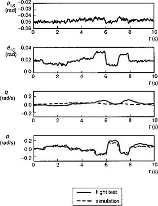
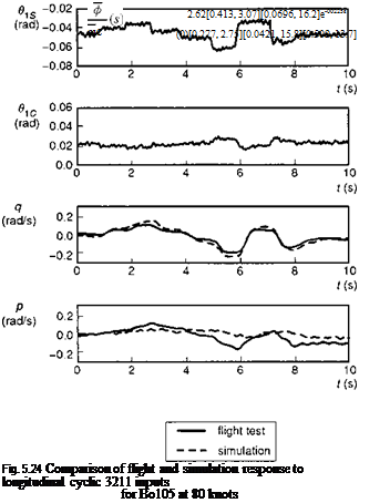
In the preceding subsections, we have seen some of the characteristics of the predicted Helisim behaviour in response to cyclic control. We complete the section with a discussion on correlation with flight test data. Figures 5.23 and 5.24 show a comparison of simulation and flight test for the Bo105 aircraft disturbed from a 80-knot trim condition. The pilot inputs are 3211 multi-steps at the lateral stick (Fig. 5.23) and longitudinal stick (Fig. 5.24); in the figures these control inputs have been transformed to the swash plate cyclics derived from sensors on the blade pitch bearings. The cyclic control signals contain harmonic components characteristic of combining
|
Table 5.3 Variation of longitudinal stability characteristics with tailplane size (Bo105 – 120 knots)
|
|
Fig. 5.23 Comparison of flight and simulation response to lateral cyclic 3211 inputs for Bo105 at 80 knots |
together individual blade angles into multi-blade form, when each blade has a slightly different mean position. The magnitude of the control inputs at the rotor is about 1° in the direct axis and about 0.3° in the coupling axis, giving an indication of the swash plate phasing on the Bo105. The comparison of the direct, or on-axis, response is good, with amplitudes somewhat overestimated by simulation. The coupled, or off – axis, response comparisons are much poorer. The swash plate phasing appears to work almost perfectly in cancelling the coupled response in simulation, while the flight data show an appreciable coupling, particularly roll in the longitudinal manoeuvre, a consequence of the low ratio of roll to pitch aircraft moments of inertia. This deficiency of the Level 1 model to capture pitch-roll and roll-pitch cross-coupling appears to be a common feature of current modelling standards and has been attributed to the absence of various rotor modelling sources including a proper representation of dynamic inflow, unsteady aero-dynamics (changing the effective control phasing) and torsional dynamics. Whatever the explanation, and it may well be different in different cases, it does seem that cross-couplings are sensitive to a large number of small effects, e. g., 5° of swash plate phasing can lead to a roll acceleration as much as 40% of the pitch acceleration following a step longitudinal cyclic input.
 |
|
Another topic that has received attention in recent years concerns the adequacy of low-order models in flight dynamics. In Ref. 5.7, Tischler is concerned chiefly with the modelling requirements for designing and analysing the behaviour of automatic flight control systems with high-bandwidth performance. Tischler used the DLR’s AGARD Bo105 test database to explore the fidelity level of different model structures for the roll attitude response (ф) to lateral cyclic stick (mc). Parametric transfer function models were identified from flight data using the frequency sweep test data, covering the range 0.7-30 rad/s. Good fidelity over a modelling frequency range of 2-18 rad/s was judged to be required for performing control law design. The least-squares fits of the baseline seventh-order model and band-limited quasi-steady model are shown in Figs 5.25 and 5.26, respectively. The identified transfer function for the baseline model is given by eqn 5.66, capturing the coupled roll/regressive flap dynamics, the regressive lead-lag dynamics, the Dutch roll mode, roll angle integration (0) and actuator dynamics, the latter modelled as a simple time delay:
 |
where the parentheses signify
[Z, o] ^ s2 + 2fos + o2, (1/T) ^ s + (1/T) (5.67)
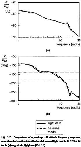
The frequencies of the Dutch roll (2.75 rad/s) androll/flap regressing mode (13.7 rad/s) compare well with the corresponding Helisim predictions of 2.64 rad/s and 13.1 rad/s, respectively. A 23-ms actuator lag has also been identified from the flight test data. From Fig. 5.25 we can see that both the amplitude and phase of the frequency response are captured well by the seventh-order baseline model.
The band-limited quasi-steady model shown in Fig. 5.26 is modelled by the much simpler transfer function given in eqn 5.68:
|
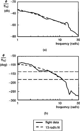
Fig. 5.26 Comparison of open-loop roll attitude frequency response; band-limited identified quasi-steady model versus flight test for Bo105 at 80 knots (Ref. 5.7): (a) magnitude; (b) phase |
The response is now modelled by a simple exponential lag, characterized by the damping derivative Lp, supplemented by a pure time delay to account for the unmodelled lags. The frequency range for which this band-limited model is valid was established by Tischler in Ref. 5.7 by identifying the frequency at which the least-squares fit error began to diverge. This occurred at a frequency of about 14 rad/s, above which the estimated parameters became very sensitive to the selected frequency. This sensitivity is usually an indication that the model structure is inappropriate. The estimated roll damping in eqn 5.68 is 14.6/s, compared with the Helisim value of 13.7/s; a total delay of over 80 ms now accounts for both actuation and rotor response. Tischler concludes that the useful frequency range for such quasi-steady (roll and pitch response) models extends almost up to the regressing flap mode. In his work with the AGARD test database, Tischler has demonstrated the power and utility of frequency domain identification and transfer function modelling. Additional work supporting the conclusions of Ref. 5.7 can be found in Refs 5.26 and 5.27.
One of the recurring issues regarding the modelling of roll and pitch response to cyclic pitch concerns the need for inclusion of rotor DoFs. We have addressed this on
many occasions throughout this book, and Tischler’s work shows clearly that the need for rotor modelling depends critically on the application. This topic was the subject of a theoretical review by Hanson in Ref. 5.28, who also discussed the merits of various approximations to the higher order rotor effects and the importance of rotor dynamics in system identification. References 5.29 and 5.30 also report results of frequency domain fitting of flight test data, in this case the pitch response of the DRA Puma to longitudinal cyclic inputs. Once again, the inclusion of an effective time delay was required to obtain sensible estimates of the 6 DoF model parameters – the stability and control derivatives. Without any time delay in the model structure, Ref. 5.29 reports an estimated value of Puma pitch damping (Mq) of -0.353, compared with the Helisim prediction of -0.835. Including an effective time delay in the estimation process results in an identified Mq of -0.823. This result is typical of many reported studies where flight estimates of key physical parameters appear to be unrealistic, simply because the model structure is inappropriate.
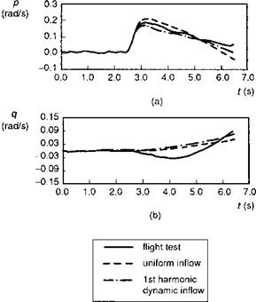
An important modelling element omitted from the forward flight Bo105 and Puma results discussed above is the effect of non-uniform dynamic inflow. We have seen from Chapters 3 and 4 that ‘unsteady’ momentum theory predicts the presence of powerful non-uniform effects in response to the development of aerodynamic hub moments. References 5.25, 5.31 and 5.32 report comparisons of predictions from blade element rotor models with the NASA UH-60 hover test database (Ref. 5.25), where the inflow effects are predicted to be strongest. The results from all three references are in close agreement. Figure 5.27, from Ref. 5.32, illustrates a comparison between flight and the
|
Fig. 5.27 Comparison of flight and simulation response to roll cyclic step, showing contribution of dynamic inflow for UH-60 in hover (Ref. 5.32): (a) roll response; (b) pitch response |
FLIGHTLAB simulation model of the response to a 1-inch step input in lateral cyclic from hover. Dynamic inflow is seen to reduce the peak roll rate response in the first half second by about 25%. The inflow effects do not appear, however, to improve the cross-coupling predictions.
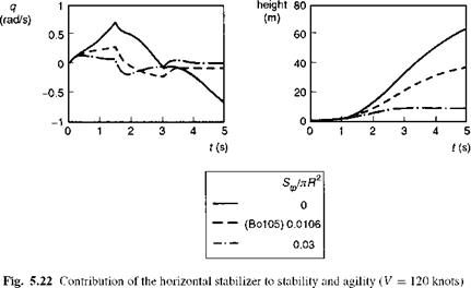
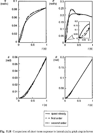
We have already seen in Figs 5.18 and 5.19 how effective the hingeless rotor can be in rolling the aircraft rapidly. This high level of controllability also applies to the pitch axis, although the accelerations are scaled down by the higher moment of inertia. Hingeless rotor helicopters are often described as agile because of their crisp attitude response characteristics. In Chapter 4 this point was emphasized by the relative magnitude of the control and damping derivatives of helicopters with different flap retention systems. We also examined stability in Chapter 4 and noted the significant decrease in longitudinal stability for hingeless rotor helicopters because of the positive pitch moment with incidence. For hingeless rotor helicopters, stability and agility clearly conflict. One of the natural ways of augmenting longitudinal stability is by increasing the tailplane effectiveness, normally achieved through an increase in tail area. The effects of tailplane size on agility and stability are illustrated by the results in Fig. 5.22 and Table 5.3. Three cases are compared, first with the tailplane removed altogether, second with the nominal Bo105 tail size of about 1% of the rotor disc area and third with the tail area increased threefold. The time responses shown in Fig. 5.22 are the fuselage pitch rate and vertical displacement following a step input of about 1° in longitudinal cyclic from straight and level trimmed flight at 120 knots. In Table 5.3 the principal aerodynamic pitching moment derivatives and eigenvalues of short-term pitch modes for the three configurations are compared. The pitch damping varies by about 10-20% from the standard Bo105 while the static stability changes by several hundred per cent.
If we measure agility in terms of the height of obstacle that can be cleared in a given time, the no-tailplane case is considerably more agile. This configuration is also very unstable, however, with a time-to-double amplitude of less than 1 s. Although not
|
|
shown in Fig. 5.22, in clearing a 50-m obstacle, the tailless aircraft has decelerated almost to the hover and rolled over by about 60° only 4 s into the manoeuvre. Pilot control activity to compensate for these transients would be extensive. At the other extreme, the large tail aircraft is stable with a crisp pitch rate response, but only manages to pop up by about 10 m in the same time. To achieve the same flight path (height) change as that of the tailless aircraft would require a control input about four times as large; put simply, the price of increased stability is less agility, the tailplane introducing a powerful stabilizing stiffness (Mw) and damping (Mq). One way to circumvent this dichotomy is to use a moving tailplane, providing stability against atmospheric disturbances and agility in response to pilot control inputs.
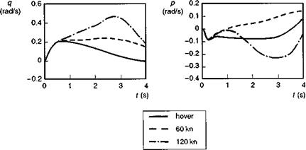
One of the characteristics of helicopters is the widely varying response characteristics as a function of forward speed. Since aircraft attitude essentially defines the direction of the rotor thrust, flight path control effectiveness also varies with speed. This adds to pilot workload especially during manoeuvres involving large speed changes. We choose the attitude response to longitudinal cyclic to illustrate the various effects. Figure 5.21 compares the pitch and roll rate response to a step cyclic input from three different trimmed flight conditions – hover, 60 and 120 knots. We have already discussed the features of the step response from hover. At 60 knots, the pitch response is almost pure rate, sustained for more than 3 s. At 120 knots, the pitch rate continues to increase after the initial transient due to the control input. This continued pitch-up is essentially caused by the strongly positive pitching moment with incidence (Mw) on the Bo105. The pitch motion eventually subsides as the speed decreases under the influence of the very high nose-up pitch attitude in this zoom climb manoeuvre. The coupled roll
|
Fig. 5.21 Variation of response characteristics with forward speed |
response has developed a new character at the high-speed condition, where the yaw response of the aircraft begins to have a stronger influence. The rotor torque decreases as the aircraft pitches up giving rise to a nose left sideslip, exposing the rotor to a powerful dihedral effect rolling the aircraft to port, and initiating the transient motion in the Dutch roll mode. Clearly, the pilot cannot fly by cyclic alone.
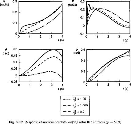
Two of the fundamental rotor parameters affecting helicopter angular motion are the effective flap stiffness, reflected in the flap frequency ratio kp, and the rotor Lock
number у, given by
The effects of these parameters on helicopter stability have already been discussed in Chapter 4, and in Chapter 2 we briefly examined the effects on dynamic response. Figures 5.19 and 5.20 compare responses to step lateral cyclic inputs for the Bol05 in hover with varying Xe and y respectively, across ranges of values found in current operational helicopters. The effect of rotor flapping stiffness is felt primarily in the short term. The initial angular acceleration decreases and the time to reach maximum roll rate increases as the hub stiffness is reduced. On the other hand, the rate sensitivity
|
|
is practically the same for all three rotors. It is also apparent that the influence of the regressing flap mode on the short-term response is reduced as the rotor stiffness decreases. To achieve an equivalent attitude response for the standard Bo105 in the first second with the two softer rotors would require larger inputs with more complex shapes. The stiffer rotor can be described as giving a more agile response requiring a simpler control strategy, a point already highlighted in Section 5.2.2. One of the negative aspects of rotor stiffness is the much stronger cross-coupling, also observed in Fig. 5.19. The strong effects of control and rate coupling (see derivatives Me1c and Mp in Chapter 4) can be seen in the pitch response of the standard Bo105 rotor configuration. The ratio of pitch attitude excursions for the three rotors after only 2 s is 7:4:1. Cross-coupling must be compensated for by the pilot, a task that clearly adds to the workload. We shall examine another negative aspect of stiff rotors later, degraded pitch stability. As always, the optimum rotor stiffness will depend on the application, but with active flight control augmentation most of the negative effects of stiffer rotors can be virtually eliminated.
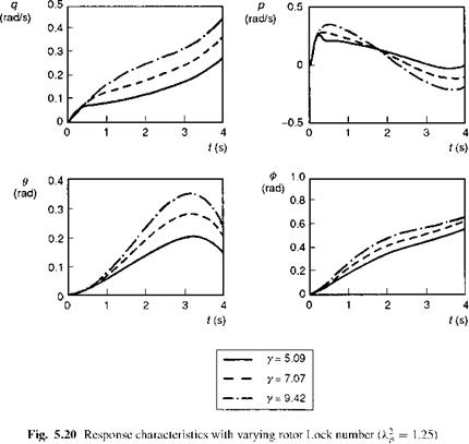
The selection of rotor Lock number is also application dependent, and the results in Fig. 5.20 illustrate the principal effects in the hover; in the cases shown, the Lock number was varied by changing the rotor blade inertia with compensating changes to rotor stiffness (Kв in eqn 5.65) to maintain constant kp. Roll control sensitivity (i. e., initial acceleration) is unaffected by Lock number, i. e., all three rotors flap by the same amount following the application of cyclic (actually the same happens for the three
|
|
rotors of different stiffness, but in those cases the hub moments are also scaled by the stiffness). The major effect of Lock number is to change the rate sensitivity, the lighter blades associated with the higher values of у resulting in lower values of gyroscopic damping retarding the hub control moment. The lower damping also increases the attitude response time constant as shown. Lock number also has a significant effect on cross-coupling as illustrated by the pitch response in Fig. 5.20.