Our heavyweight helicopter equal in the world does not have
In Rostov started production of the most load-lifting rotary-wing car The Russian holding «Helicopt[...]

Everything about aircrafts and helicopters. News and events in aviation worldwide. Civil, transportation, military helicopters and airplanes.

Everything about aircrafts and helicopters. News and events in aviation worldwide. Civil, transportation, military helicopters and airplanes.

Everything about aircrafts and helicopters. News and events in aviation worldwide. Civil, transportation, military helicopters and airplanes.

Everything about aircrafts and helicopters. News and events in aviation worldwide. Civil, transportation, military helicopters and airplanes.


A control malfunction occurs when the control surface does not move consistently with the input, and in this section the failure corresponding to an actuator moving ‘hard-over’ to its limit is considered. The effect of such a failure in the longer term is likely to be that the actuator is disengaged, although it does not necessarily follow that the control function is then ‘lost’. The failure may be in a limited-authority actuator, feeding augmentation signals to the control surface in series with the pilot’s inputs. The loss of this function is unlikely to be flight critical although it may be mission critical. For example, the loss of control augmentation may reduce the handling qualities in degraded visual conditions from Level 1 to Level 3 (e. g., loss of TRC sensor systems degrading response type to RC in a UCE = 3). The aircraft is still controllable but should the pilot attempt any manoeuvring close to the ground, the high risk of loss of spatial awareness would render the operation unsafe. If the actuator forms part of the primary flight control system then it would be normal to have sufficient redundancy so that a back-up system is brought into play to retain the control function following the failure. The question then becomes how much of a failure transient can be tolerated before the back-up system takes over? Similarly, how much failure transient can be tolerated before a runaway augmentation function is made safe? The transient response of the aircraft to failures therefore becomes part of the FMEA. ADS-33 (Ref. 8.3) addresses the consequences of these transients in a threefold context – possible loss of control, exceedance of structural limits and collision with nearby objects. Table 8.7 summarizes the requirements in terms of attitude excursions, translational accelerations and proximity to the OFE. The hover/low-speed requirements are based on the pilot being in a passive, hands-on state, perhaps engaged with other mission-related tasks. The 3-s intervention time then takes account of pilot recognition and diagnosis of the failure, before initiating the correct recovery action. The Level 3 requirements relate to the aircraft having been disturbed about 50 ft from its hover position before the pilot reacts. The assumption is that in such circumstances, the aircraft would have collided with surrounding obstacles or the ground. The Level
|
Table 8.7 Failure transient requirements (ADS-33)
|
2 and Level 1 requirements then provide increasing margins from this ‘loss of control’ situation.
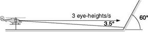
References 8.46 and 8.47 both deal with failure transients and degraded flying qualities of tilt rotor aircraft. In Ref. 8.46, the methodology for dealing with loss, malfunction and degradation in the development of the European Civil Tilt Rotor is described. Reference 8.47 is concerned with the V-22 and will be returned to later in this section. In Ref. 8.46, the up-and-away requirements for the civil tilt rotor were expressed in terms of the transient attitude excursions following a failure, shown in Table 8.8, with the assumption that the pilot was hands-off the controls and would require 3.5 s to initiate recovery action (Ref. 8.48).
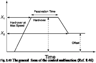
Degradation into Level 4 handling qualities would result from attitude transients shown with the consequent high risk of loss of spatial awareness and hence control. An analysis was conducted using the civil tilt rotor simulation model to establish the handling qualities boundaries as a function of the parameters of the hard-over as summarized in Fig. 8.40. The control surface is driven at the maximum actuation rate to a value X1, which is then held for the so-called passivation time, after which the surface returns to an offset value X2.
Figure 8.41 shows results for the roll angle following a failure of the left aileron to 16° initiated at 0.1 s. For the case shown, the aileron reached the failure limit, driven at the maximum actuation rate, in 0.4 s. The aileron holds the hard-over position for the passivation time of 1.5 s, after which the surface is returned to an offset value of 3° at the reduced rate of the back-up system. The pilot takes control at 3.5 s, applying full right aileron and achieving this in 1 s (reduced actuation rate of 100%/s). In the example
Table 8.8 Failure transient requirements (Ref. 8.46)
Transient attitude excursions; forward flight, up-and-away
Level 1 20° roll, 10° pitch, 5° yaw
Level 2 30° roll, 15° pitch, 10° yaw
Level 3 60° roll, 30° pitch, 20° yaw
Time (s)
 |
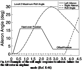 |
shown, the maximum roll angle of 30° occurred at about 3 s and the transient response was already reducing by the time the pilot applied corrective action. In the study reported in Ref. 8.46, the failure parameters in Fig. 8.40 were varied to define the handling qualities boundaries according to Table 8.8, using the methodology typified in Fig. 8.41. In this way the designer can use the results to establish the required safety margins in the design that guarantee that the handling stays within the Level 1 or Level 2 regions.
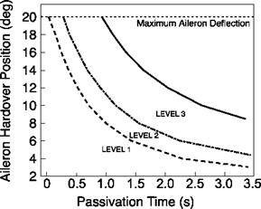
Figure 8.42 shows the handling qualities regions using the two-parameter chart of maximum aileron deflection versus passivation time. The results are shown for the zero offset condition. So, for example, with a passivation time of 1.5 s, the Level 3 boundary is reached with failure amplitude of about 15°. The methodology allows a wide range of different scenarios to be assessed. Cases where the failed actuator is not
|
Fig. 8.42 Handling qualities levels for roll response shown as a function of passivation time and aileron hard-over amplitude (Ref. 8.46) |
returned to an offset can also be considered, as can cases where the failure magnitude is limited to the authority of the in-series, stability augmentation.
The recovery control action discussed above is formulated clinically as shown in Fig. 8.40 and with the very large number of test cases needing quantification, off-line production of the knowledge contained in charts like Fig. 8.42 is the only realistic approach. The results derived from such analysis provide the ‘predicted’ handling qualities. But, as with flying qualities testing in normal conditions, piloted tests are required to support and validate the analysis. It has become a normal practice in some qualification standards to require flight testing to be carried out, e. g., SCAS failures in the UK Defence Standard (Ref. 8.42), but in most cases, the risk to flight safety is so high that such testing is actually never carried out, particularly addressing the question – what impact does the degradation have on flying qualities post-failure? In Ref. 8.47, the methodology adopted during qualification of the V-22 flying qualities is described, wherein extensive use of piloted simulation was made to answer this question. Following the recovery from the failure transient, it is expected that this aircraft will need to fly the equivalent of MTEs even in fly-home mode, although some may be impossible to set up. Reference 8.47 highlights the importance of maintaining the same performance standards as when flying operationally without failures. To quote from Ref. 8.47,
Relaxing task requirements can open the possibility of a very undesirable dilemma: the severely crippled aircraft could receive HQRs that are not much worse than, or possibly are even better than, those for the unfailed aircraft. For the precision hover example, suppose the performance limits were relaxed from ‘hover within an area that is Xfeet on each side’ to ‘don’t hit the ground’. Precision hover is typically more difficult in the simulator than inflight, so Level 2 HQRs (4, 5, or 6) would not be surprising for the unfailed aircraft performing the tight hover MTE. Artificially opening the performance limits, to accommodate the presence of the failure, could lead a pilot to assign a comparable – or better – HQRfor what might be an almost uncontrollable configuration.
So, the extent of the handling degradation following system failures can be properly measured only through a direct comparison with the unfailed aircraft, using both predictive (off-line) and assignment (pilot assessment) methods.
It is also important to establish the pilot’s impressions of the transient effect of the failure and ability to recover, aspects not covered by a handling rating per se. The failure rating scale developed by Hindson, Eshow and Schroeder (Ref. 8.49) in support

Ability to Recover Rating
Tolerable
 |
|
Intolerable
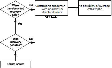
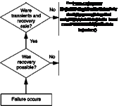
Fig. 8.43 Failure transient and recovery rating scale
of the development of an experimental fly-by-wire helicopter was modified in the V-22 study, and this version is reproduced here as Fig. 8.43. The essential modifications relative to the original Ref. 8.49 scale were firstly the nature of the questions on the left-hand side; positive answers moved up the scale, as in the Cooper-Harper handling qualities scale. Secondly, the exceedances in failure categories A to F were referred to the safe flight envelope (SFE) rather than the OFE, and thus to effectively maintain Level 2 handling qualities.
 |
 |
|
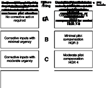
Pilots rate two aspects of the failure using Fig. 8.43 – the effect of the failure itself and the consequent ability to recover to a safe equilibrium state. Failure ratings (FR) A to E would be regarded as tolerable, F to G as intolerable, with a marginal recovery capability, while a rating of H means there is ‘no possibility of averting a catastrophe’. In the programme to develop the European civil tilt rotor this methodology has been extended to produce an integrated classification of failures as illustrated in Fig. 8.44 (Ref. 8.50) and is itself an extension of that adopted in the development and certification of the NH-90 helicopter. The integration brings together the failure category concept (minor-catastrophic), the FR and the HQR. In Fig. 8.44, the OFE exceedance requirements were maintained corresponding to failures A to E rather than the SFE modification in Ref. 8.47. We can see that a ‘minor’ failure that elicits an FR
Fig. 8.44 Integrated classification of failures
of A or B results in the aircraft maintaining its Level 1 handling qualities. If the ratings degrade to C or D, the aircraft falls into the Level 2 category. Major failures correspond to degradations to Level 3 handling qualities while Hazardous or Catastrophic failures correspond to the aircraft being ‘thrown into’ the Level 4 region where loss of control is threatened.
The integration is considered to offer an important new framework for relating the impact of flight system failures on flight handling qualities, within which engineers and pilots can develop and qualify systems that are safe.
As discussed above, a malfunction can often lead to a loss of control function, but we need now to consider the third failure type where the control function is still operating but with degraded performance.
Loss of control is a most serious event, and huge emphasis on safety in the aviation world is there to ensure that all possible events that might lead to a loss of a flight critical function are thoroughly examined and steps taken in the design process to ensure that such losses are extremely improbable. In military use, when helicopters can be exposed to the hazards of war, steps are sometimes taken to build in additional levels of redundancy in case of battle damage. For example, the AH-64 Apache features a back-up, fly-by-wire control system that can be engaged following a jam or damage in the mechanical control runs. The tail rotor is particularly vulnerable to battle damage, and a study carried out by DERA and Westland for the UK MoD and CAA, during the mid-late 1990s, identified that tail rotor failures occur in training and peace-time operations at a rate significantly higher than the airworthiness requirements demand. In the following section some of the findings of that study are presented and discussed.
Tail rotor failures
We broaden the scope to include both types of tail rotor failure: drive failure, where the drive-train is broken and a complete loss of tail rotor effectiveness results, and control failure, where the drive is maintained but the pilot is no longer able to apply pitch to the tail rotor. Both examples result in a loss of the yaw control function and can occur because of technical faults or operational damage. References 8.43 and 8.44 describe a programme of research aimed at reviewing the whole issue of tail rotor failures and developing improved advice to aircrew on the actions required, following a tail rotor failure in flight. The activity was spurred by the findings of the UK MoD/CAA Tail Rotor Action Committee (TRAC), which in particular were as follows (Ref. 8.9):
(a) Tail rotor failures occur at an unacceptably high rate. MoD statistics between 1974 and 1993 showed a tail rotor technical failure rate of about 11 per million flying hours; the design standards require the probability of transmission/drive failure that would prevent a subsequent landing to be remote (<1 in a million flying hours, Ref. 8.42); a review of UK civil accident and incident data revealed a similar failure rate.
(b) Tail rotor drive failures are three times more prevalent than control failures.
(c) There appear to be significant differences in the handling qualities post-tail rotor failure, between different types (e. g., some designs appeared to be uncontrollable,
and the probability of an accident resulting from a failure is greater with some types
than others), although there is a dearth of knowledge on individual types.
(d) Improved handling advice would enhance survivability.
TRAC recommended that work should be undertaken to develop validated advice for pilot action in the event of a tail rotor failure for the different types in the UK military fleet, and also that airworthiness requirements should be reviewed and updated to minimize the likelihood of tail rotor failures on future designs. In the study that followed, validation was classified into three types – validation type 1 corresponding to full demonstration in flight, validation type 2 corresponding to demonstration in piloted simulation combined with best analysis and validation type 3 corresponding to engineering judgement based on calculation and also read-across from other types. It was judged that the best advice that could be achieved would be supported by type 1 validation for control failures and type 2 validation for drive failures.
The study, reported fully in Ref. 8.44, drew data from a variety of sources including the MoD and CAA, the US Navy, Marine Corps and Coast Guard and the US National Transport Safety Board (NTSB). The overall failures rates were relatively consistent across all helicopter ‘fleets’ and occurred in the range 9-16 per million flying hours. Recall that civil transport category aircraft are required to have a failure rate for flight critical components of no more than 1 in 109 flying hours. Of the 100 ‘tailfails’ in the UK helicopter fleet between the mid-70s and mid-90s, 30% were caused by drive failure and 16% by control failure or loss of control effectiveness. Tail rotor loss due to collision with obstacle or vice versa accounted for 45% of the failures.
When investigating flying qualities in failed conditions, two different aspects need to be addressed – the characteristics during the failure transient and post-failure flying qualities, including those during any emergency landing. Both are, to some extent, influenced by the flight condition from which the failure has occurred. For example, the failure transients and optimum pilot actions will be quite different when in a low hover compared with those in high-speed cruise, well clear of the ground. The required actions will also be different for drive and control failures. Furthermore, in the case of control failures, the aircraft and appropriate pilot responses will depend on whether the control fails to a high pitch or low pitch, or some intermediate value, perhaps designed in as a fail-safe mechanism to mitigate the adverse effects of a control linkage failure.
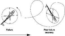
Reference 8.44 describes a flight trial, using a Lynx helicopter, where control failures were ‘simulated’ by the second pilot (P2) applying pedals to the failure condition. P2 held the failed condition, while P1 endeavoured to develop successful recovery strategies using a combination of cyclic and collective. The high-pitch control failure mode results in a nose-left yaw (for anti-clockwise rotors), the severity of which depends on the initial power setting and aircraft speed. For example, the magnitude of control and yaw excursions will be greater from flight at minimum power speed than cruise. Accompanying the yaw will be roll and pitch motions, driven by the increasing sideslip. In the flight trials, a number of different techniques were explored to recover the aircraft to a stable and controllable flight condition. For failures in highspeed cruise, attempts to decelerate through the power bucket to a safe-landing speed were unsuccessful; the right sideslip (left yaw) built up to limiting values, and controlling heading with cyclic demanded a very high workload. A successful strategy was developed as illustrated in Fig. 8.38.
|
|
|
|
||||
|
|||||||
|

![]()
A high-power climbing turn to the left gave a sufficiently stable flight condition so that deceleration could be accomplished without the aircraft diverging in yaw. The aircraft could then be levelled out at about 40 knots and a slow decelerating descent initiated. Gentle turns to both right and left (left preferred) were possible in this condition. The landing was accomplished by lining the aircraft up with the nose well to port and applying collective, and levelling the aircraft, just before touchdown to arrest the rate of descent and align the aircraft with the flight path. Running landings between 20 and 40 knots could be achieved with this strategy. In comparison, low thrust control failures resulted in the aircraft yawing to starboard. Reducing power then arrests the yaw transient and allows the aircraft to be manoeuvred to a new trimmed airspeed. During recovery it was important that the pilot yawed the aircraft with collective to achieve a right sideslip condition, so that collective cushioning prior to landing yawed the aircraft into the flight path.
 |
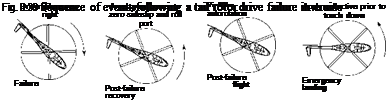 |
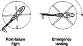
The drive failures were conducted in the relative safety of the DERA advanced flight simulator (see Chapter 7, Section 7.2.2). The trial was conducted within the broad framework of the flying qualities methodology with task performance judged by the pilot’s ability to land within the airframe limits, i. e., touchdown velocities and drift angle. Unlike a control failure, where the tail rotor continues to provide directional stability in forward flight, in a drive failure this stability augmentation reduces to zero as the tail rotor runs down. For failures from both hover and forward flight, survival is critically dependent on the pilot recognizing the failure and reducing the power to zero as quickly as possible. Figure 8.39 shows the sequence of events following a drive failure from a cruise condition. The aircraft will yaw violently to the right as tail
rotor thrust reduces. The study showed that a short pilot intervention time is critical here to avoid sideslip excursions beyond the structural limits of the aircraft. The pilot should reduce power to zero as quickly as possible by lowering the collective lever. Once the yaw transients have been successfully contained, and the aircraft is in a stable condition, the engines can be shut down and the aircraft retrimmed at an airspeed of about 80 knots. With the Lynx, this gives about a 20% margin above the speed where loss of yaw control is threatened. Any attempt to find a speed-power combination that enabled continued powered flight risked a yaw breakaway which could drive the aircraft into a flat spin. Gentle turns to right and left (more stable) were possible from the 80 knots autorotation. The pilot approaches the landing with the aircraft nose to starboard and, in this case, raising collective to cushion touchdown yaws the nose to port and aligns with the flight path.
Reference 8.44 describes typical examples of tail rotor failure that were in the database investigated. One such example involved a Lynx helicopter taking off on a test flight following the fitting of a new tail rotor gearbox. With the aircraft in a low hover, a ‘low power’ control failure occurred. To quote from Ref. 8.44,
As the aircraft lifted there was a slight yaw to the right which the pilot compensated for, but by the time the aircraft was established in a 10feet hover, a matter of only 2-3 seconds after launch, the aircraft was continuing to diverge to the right with full left pedal applied. The pilot called out full left pedal’, and the aircraft accelerated into a right hand spot turn over which the aircrew had no control. The aircrew recalled the AEO’s briefing and reduced the MR speed (which also reduced tail rotor speed and thrust), the yaw accelerated further, exacerbated by the fact that they were entering the downwind arc. The words of the briefing were then recalled ‘right hand turn equals low power setting, therefore increase NR’. The speed select lever was pushed forward to increase MR speed (and hence tail rotor speed and thrust), the yaw rate slowed down. The aircrew regained control of the aircraft and were able to land without further incident.
The Aircraft Engineering Officer (AEO) referred to here had actually led the tail rotor flight and simulation programme at DERA and is the first author of Ref. 8.43, and hence was very familiar with tail rotor failures. He had briefed the maintenance flight aircrew on actions to take in the event of a tail rotor failure. The advice proved crucial and the pilot’s actions averted a crash; the story is told in Ref. 8.45.
Reference 8.44 also identifies a number of candidate technologies that could mitigate the effects of tail rotor failure, e. g., warning systems, integrated with health and usage monitoring systems, emergency drag parachutes. This is an important line of development in the context of safety. The accident data highlight that drive failures on most types are not very survivable. The two illustrations used to describe the failure types show a straightforward transition from the failure through the recovery to the landing. In practice, however, the pilot is likely to be confused initially by what has happened (note above example where the pilot operated the speed select lever in the wrong direction initially) and can quickly become disoriented as the aircraft not only yaws, but also rolls and pitches, as sideslip builds up. Also, the accident/incident data show that on several occasions the pilot has successfully recovered from the failure but the aircraft has turned over during the landing. Tail rotor failures make undue demands on pilot skill and attention and the way forward has to be to ensure that designs have sufficiently reliable drive and control systems so that the likelihood of component failure is extremely remote in the life of a fleet. Reference 8.44 recommends that the Joint Aviation Requirements be revised to provide a two-path solution to ‘closing the regulatory gap’ in respect of tail rotor control systems. Firstly, fixed-wing aircraft levels of redundancy of flight critical components are required. Secondly, where redundancy may be impractical, ‘the design assessment should include a failure analysis to identify all failure modes that will prevent continued safe flight and landing and identification of the means provided to minimise the likelihood of their occurrence’.
Reference 8.44 also recommended that the ADS-33 approach of specifying failure transients (see next section) be adopted along with the collective to yaw coupling requirements and sideslip excursion limitations as a method of quantifying the effects of failure. Such criteria could also form the basis for evaluating the effectiveness of retrofit technologies, including contributions from the automatic flight control system. Tail rotor failures require the pilot to exercise supreme skill to survive what is, quite simply, a loss of control situation. If flying qualities degradation could be contained within the Level 3 regime, with controllability itself not threatened, then the probability of losing aircraft to such failures would be reduced significantly. Time will tell how effectively the recommendations of Ref. 8.44 are taken up by the Industry.
The structure of Flying Qualities Levels provides the framework for analysing and quantifying the effects in the event of a flight system failure. Failures can be described under three headings – loss, malfunction or degradation – as described below:
(a) Loss of function: for example, when a control becomes locked at a particular value or some default status, hence where the control surface does not respond at all to a control input;
(b) Malfunction: for example, when the control surface does not move consistently with the input, as in a hard-over, slow-over or oscillatory movement;
(c) Degradation offunction: in this case the function is still operating but with degraded performance, e. g., low-voltage power supply or reduced hydraulic pressure.
The first stage in a flying qualities degradation assessment involves drawing up a failure hazard analysis table, whereby every possible control function (e. g., pitch through longitudinal cyclic, yaw through tail rotor collective, trim switch) is examined for the effects of loss, malfunction and degradation. This assessment is normally conducted by an experienced team of engineers and pilots to establish the failure effect as minor, major, hazardous or catastrophic. Table 8.4 summarizes the definitions of these hazard categories in terms of the effects of the failure and the associated allowable maximum probability of occurrence per flight hour (Ref. 8.40). The table refers to the system safety requirements for civil aircraft.
In the military standard ADS-33, the approach taken is defined in the following steps (Ref. 8.3) (author’s italics for emphasis):
(a) tabulate all rotorcraft failure states (loss, malfunction, degradation),
(b) determine the degree of handling qualities degradation associated with the transient for each rotorcraft failure state,
(c) determine the degree of handling qualities degradation associated with the subsequent steady rotorcraft failure state,
|
Table 8.4 Failure classification
|
(d) calculate the probability of encountering each identified rotorcraft failure state per flight hour,
(e) compute the total probabilities of encountering Level 2 and Level 3 flying qualities in the Operational and Service Flight Envelopes. This total is the sum of the rate of each failure only if the failures are statistically independent.
Degradation in the handling qualities level, due to a failure, is permitted only if the
probability of encountering the degraded level is sufficiently small. These probabilities shall be less than the values shown in Table 8.5. The probabilities used in ADS-33 are based on the fixed-wing requirements in Ref. 8.41, but converted from the probability per flight to the probability per flight hour, with the premise that a typical fixed – wing mission lasts 4 h. The requirements are not nearly as demanding as the civil requirements of Table 8.4 where the probabilities are typically two orders of magnitude lower.
In contrast, the UK Defence Standard (Ref. 8.42) defines safety criteria for failures of automatic flight control systems (AFCS) according to Table 8.6. The effect is defined
|
Table 8.5 Levels for rotorcraft failure states |
|
|
Probability of encountering failure |
|
|
Within operational flight envelope |
Within service flight envelope |
|
Level 2 after failure <2.5 x 10⁻³ per flight hour Level 3 after failure <2.5 x 10⁻⁵ per flight hour Loss of control <2.5 x 10⁻⁷ per flight hour |
<2.5 x 10⁻³ per flight hour |
|
Table 8.6 AFCS failure criteria (Def Stan 00970, Ref. 8.42)
|
within the so-called intervention time, which is a function of the pilot attentive state. With the pilot flying attentive hands-on, for example, the intervention time is 3 s, but in passive hands-on mode, the time increases to 5 s.
In the following sections, examples are given of failures in the three categories along with results from supporting research.
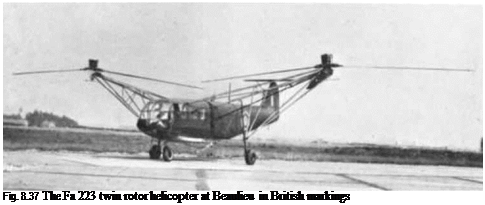
The second issue of the Journal of the Helicopter Society of Great Britain, published in 1947, featured just two papers. The first was by Sikorsky and has already been referred to in the Introduction to this chapter (Ref. 8.1). The second was by O. L.L. Fitzwilliams, or ‘Fitz’ as he was affectionately known to his colleagues at Westland Helicopters, where he worked at the time of writing the paper in late 1947. Fitz had previously worked at the Airborne Forces Experimental Establishment at Beaulieu, near Southampton, England, during the Second World War and his paper partly covered his experiences there, including tests conducted on German rotorcraft acquired during the closing stages of the war. One such type was the first production helicopter (Ref. 8.37) – the Focke-Achgelis Fa 223, a development of the first practical helicopter, the FW.61. The Fa 223 aircraft was flown ‘by its German crew, via Paris, to the A. F.E. E., at Beaulieu, where it arrived in September 1945, having performed the first crossing of the English Channel by a helicopter’. The Fa 223 was a twin rotor configuration with longitudinal cyclic control for pitch and differential collective for roll. Differential longitudinal cyclic gave yaw control in hover, supplemented by the rudder in forward flight. All these functions are nowadays to be found on a modern tilt rotor aircraft. More details of the flight control system on the Fa 223 are reported in Refs 8.38 and 8.39. Figure 8.37, from Ref. 8.39, shows a photograph of the aircraft at Beaulieu.
The handling qualities problems of the Fa 223 largely stemmed from the mechanism for lift control – essentially throttle and rotorspeed, which resulted in major deficiencies. To quote from Ref. 8.39,
In hovering or in low speed flight, the control of the lift by means of the throttle is extremely sluggish and has contributed to the destruction of at least one aircraft following a downwind turn after take off. Moreover, the sluggishness of the lift control necessitates a high approach for landing and a protracted landing manoeuvre, during which the aircraft is exposed to the dangers consequent on operation of the change mechanism.
The ‘change mechanism’ allowed the pilot, via a two-position lever, to change the mean blade pitch to its helicopter position (up) or its autorotation position (down). Lowering the lever caused the engine clutch to be disengaged, and the rotor blades rotate at a controlled rate (via a hydraulic ram and spring) to the autorotative pitch setting. This mechanism operated automatically in the event of engine failure, transmission failure and a number of other ‘failure modes’, some of which appear not to have been fully taken into account during design (Ref. 8.39). The failure mechanism was also irreversible and Fitz recounts his experience during an early flight test with the aircraft, when an auxiliary drive failure caused an automatic change to the autorotative condition (Ref. 8.37).
Once the mechanism had operated, even voluntarily, it was impossible to regain the helicopter condition in flight and a glide landing was necessary. In fact, with the high disc loading of this aircraft (author’s note; 5.9 lb/ft2 at 9,500 lb) and the absence of any control over the blade pitch, a glide landing was essential and if there was not enough height for this purpose the operation of this so-called safety mechanism would dump the aircraft as a heap of wreckage on to the ground. This actually happened, at about 60-70 ft above the ground, shortly after the machine arrived at Beaulieu, and I was among those who were sitting in it at the time. In consequence, I have a strong prejudice against trick gadgets in helicopter control systems and also a rooted objection to helicopters, however light their disc loadings, which do not allow the pilot direct manual control over the blade pitch in order to cushion a forced landing.
Although the Fa 223 first flew in August 1940, at the cessation of hostilities only three aircraft existed and the loss of the aircraft at Beaulieu brought to a premature end to the testing of what was undoubtedly a remarkable aircraft with a number of ingenious design features, notwithstanding Fitz’s prejudices.
Nowadays, the safety assessment of this design through a failure modes and effects analysis (FMEA) would have deemed the consequences of this failure mode close to the ground ‘catastrophic’, and a greater reliability would be required in the basic design. An engine failure at low altitude would have been equally catastrophic of course, without control of collective pitch, as Fitz implied, but this is no justification
for having a safety device that itself had a hazardous failure mode. In handling qualities terms, the failure, at least while the aircraft was in hover close to the ground, resulted in degradation to Level 4 conditions, the pilot effectively losing control of the aircraft. In the Introductory Tour to this book in Chapter 2, the author cited another example of a helicopter being flown in severely degraded handling qualities. The cases of the S.51 and the Fa 223 are highlighted not to demonstrate poor design features of early types (hindsight offers some clarity but usually fails to show the complete picture), but rather to draw to the reader’s attention to the way in which the helicopter brought new experiences to the world of aviation, 40 years after the Wright brothers’ first flight, at a time when ‘flying qualities’ was in its infancy and still a very immature discipline. But a holistic discipline it would become, spurred by the need for pilots and engineers to define a framework within which the performance increases pursued by operators, for commercial or military advantage, could be accommodated with safety. How to deal with failures has always been an important part of this framework and we continue this chapter with a discussion of current practices for quantifying flying qualities degradation following failures of flight system functions.
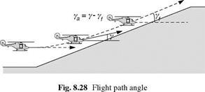
For the t analysis, the aircraft flight path angle у is converted to ya, the negative perturbation in у from the final state, as illustrated in Fig. 8.28.
If the aircraft’s normal velocity w is small relative to the forward velocity V, the flight path angle can be approximated as
w
Y *-y (8.35)
If the final flight path angle is yf, then the y-to-go, Ya can be written as
![]()
Ya = Y – Y f
|
|
|
|
|
|
|
|
|
|
Fig. 8.29 ya, ya during the climb |
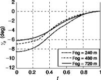
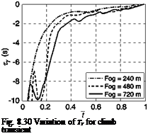
The y’s-to-go and associated time rates of change are plotted in Fig. 8.29 for the UCE = 1 and UCE = 2 fog-line cases, although it should be noted that the 240-m case is actually borderline UCE = 2/UCE = 3. In Fig. 8.29, time has been normalized by the duration of the climb transient (fog = 240 m, T = 2.5 s; fog = 480 m, T = 4.3 s; fog = 720 m, T = 4.7 s). The final value of the flight path angle was chosen as the value when Y first became zero (thus defining T and yf); hence, although the hill had a 5° slope, the values used correspond to the first overshoot peak value. From that time on, the pilot closes the loop on a new т gap, related to the flight path error from above. As can be seen from the initial conditions, the pilot tends to overshoot the 5° hill slope with increasing extent as the UCE degrades – flight path angle of 8.5° for the 240-m fog-line (UCE 2/3), 7° for the 480-m fog-line case (UCE 2) and 6° for the 720-m case (UCE 1).
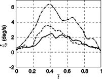
Figure 8.30 shows the variation of Ty with normalized time. The fluctuations reflect the higher frequency content in the Y function. As the goal is approached the curves straighten out and develop a slope of between 0.6 and 0.7, corresponding to the pilot following the т constant guide with peak deceleration close to the goal.
As with the accel-decel manoeuvre, the pilot is changing from one state to another (horizontal position for the accel-decel, flight path angle for the climb), and as discussed earlier, the natural guide for ensuring that such changes of state are achieved successfully is the constant acceleration guide, with the relationship, Ty = кTg.
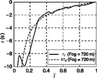
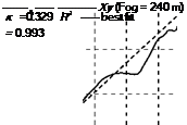
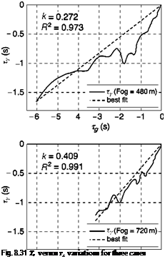
Figure 8.31 shows results for the Ty versus Tg correlation for the terrain climb in the three fog conditions. In the UCE = 1 case (720 m fog), apart from a slight departure at the end of the manoeuvre, the fit is tight for the full 5 s (R2 = 0.99). The departures from the close fit at both the beginning and end of such state change
 |
manoeuvres are considered to be transient effects, partly due to the need for the pilot to ‘organize’ the visual information so that the required gaps are clearly perceived and partly due to the contaminating effects of the pitch changes that disrupt the visual cues for flight path changes picked up from the optic flow. Table 8.3 gives the coupling coefficients, k, for all cases flown. The lower the k value, the earlier in the manoeuvre the maximum motion gap closure rate occurs (e. g., a value of 0.5 corresponds to a symmetric manoeuvre). There is a suggestion that k reduces as UCE degrades, confirmed by the results in Fig. 8.31. The pilot has commanded a flight path angle rate of about 6°/s less than 40% into the manoeuvre in the UCE = 2-3 case compared with about 2.5°/s about 50% into the manoeuvre in the UCE = 1 case.
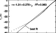
Typical correlations between xy and Tg are shown in Fig. 8.32, plotted against normalized time. The relatively constant slope during the second half of the manoeuvre indicates that the pilot has adopted a constant T strategy. As expected, the test data track the constant acceleration guide fairly closely over the whole manoeuvre.
The results reveal a strong level of coupling with the T guide. This was not unexpected. In a complementary study, t analysis has been conducted on data from approach and landing manoeuvres for fixed-wing aircraft (Ref. 8.30). During the landing flare, the pilot follows the T guide to the touchdown. Instrument approaches where the visibility was reduced to the equivalent of Cat IIIb (cloud base 50 ft, runway visual range 150 ft) were investigated, and in some cases the coupling reached the limiting case of constant t, the pilot effectively levelling off just above the runway. The results presented are consistent with those presented in Ref. 8.30, unsurprisingly as the flare and terrain climb tasks make very similar demands on the pilot in terms of visual information.
From eqns 8.34 and 8.35, we can write the equation for flight path perturbation dynamics as
with
![]() Ya (t = 0) = – Yf
Ya (t = 0) = – Yf
 |
-6 -5 -4 -3 -2 -1 О
 |
Tg(s)
-6 -5 4 -3 -2 -1 О
*(s)
|
Table 8.3 Correlation constants and fit coefficients – following the constant acceleration guide
|
![]()
|
|
|
|
|
|
|
|
|
|
|
|
The instantaneous time to reach the goal of у = уf is defined as
Ty a = — (8.41)
Ya
Following a t guide such that tx = kTg results in motion that follows the guided motion as a power law
x = Cxg1 к (8.42)
where C is a constant.
Recapping from earlier in the chapter, the constant acceleration guide has the forms given by
agis the constant acceleration of the guide. As discussed earlier and shown in Fig. 8.21, the motion begins and ends hand-in-hand with the guide, but initially overtakes before being caught up and passed by the guide at the goal.
The equations for the flight path motion and its derivatives can then be developed (see Ref. 8.24) and written in the normalized form
![]()
![]() Ya = ? a -12)( 1 -1)
Ya = ? a -12)( 1 -1)
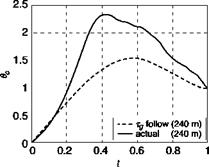
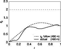
From eqn 8.39, the collective control can then be written in the general form в 0 = 1 + ta Y a + Y a
Combining with eqns 8.45 and 8.46, the normalized collective pitch is given by the expressions
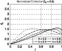
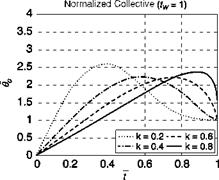
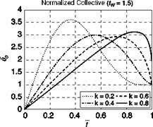
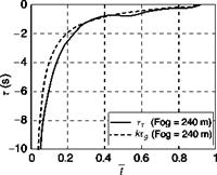
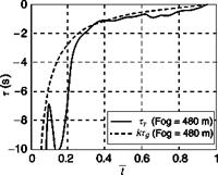
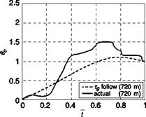
The normalized functions в0 and Ya(independent of tw ) are plotted in Figs 8.33 and 8.34, as a function of normalized time for different values of coupling constant k. The three cases correspond to the parameter tw set at 0.5,1.0 and 1.5. The strategy involves increasing the collective gradually, and well beyond the steady-state value, and then decreasing as the target rate of climb is approached. For tw = 0.5, when the heave time constant is half the manoeuvre duration, the overdriving of the control is limited to about 50% of the steady-state value. As the ratio increases to 1.5, so too does the overdriving to as much as 250% at the lower k values. This overshoot is unlikely to be achievable even when operating with a low-power margin. As k increases, the peak
|
|
|
|
|
Fig. 8.33 Normalized collective pitch for a flight path angle change following a constant acceleration т guide – variations with k and tw |
collective lever position occurs later in the manoeuvre until the limiting case where it is reduced as a down-step in the final instant to bring Ya to zero. When approaching a slope, the pilot has scope to select T, hence tw, and k, to ensure that the control and hence the manoeuvre trajectory are within the capability of the aircraft. Whatever values are selected, the control strategy is far removed from the abrupt, open-loop character associated with a step input.
|
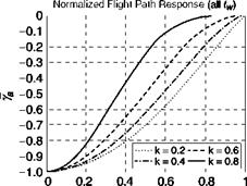
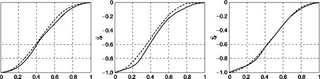
t Fig. 8.34 Normalized flight path response for a flight path angle change following a constant acceleration т guide-variations with k |
A comparison of normalized collective inputs and flight path angles with the т-coupled predictions for representative cases is shown in Fig. 8.35. The large peak for the 240-m fog-line case resulted in the overshoot to 10° flight path angle discussed earlier and could be argued in a case where the pilot has lost track of the cues that enable the т – coupling to remain coherent. The actual pilot control inputs appear more abrupt than the predicted values but it again could be argued that the pilot needs to stimulate the flow-field initially with such inputs. There is good agreement for the flight path angle variations.
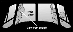
In Ref. 8.31, the notion was put forward that ‘the overall pilot’s goal is to overlay the optic flow-field over the required flight trajectory – the chosen path between the trees, over the hill or through the valley – thus matching the optical and required flight motion’. This concept can be extended to embrace the idea that the overlay technique can happen within a temporal as well as spatial context. The results presented above convey a compelling impression of pilots coupling onto a natural т guide during the 3-5 s of the climb phase of the terrain-hugging manoeuvre. As in the accel-decel manoeuvre, pilots appear to pick up their visual information from about 12 to 16 eye – heights ahead of the aircraft and establish a flight speed that gives a corresponding look-ahead time of about 6-8 s. As height is reduced, the pilot slows down to maintain velocity in eye-heights, and corresponding look-ahead time, relatively constant. The manoeuvre is typically initiated when the Tsurface reduces to about 6 s and takes between 4 and 5 s to complete. Of course, the manoeuvre time must depend on the heave time constant of the aircraft being flown. For the FLIGHTLAB Generic Rotorcraft simulation model used in the trials, tw varies between 3 s in hover and 1.3 s at 60 knots, reducing to below 1 s above 100 knots. Much stronger interference between the aircraft and task dynamics would be expected with aircraft that exhibited much slower heave response (e. g., aircraft featuring rotors with high-disc loadings), as illustrated in Fig. 8.32.
The temporal framework of flight control offers the potential for developing more quantitative UCE metrics. For example, in the terrain manoeuvres described above, the UCE = 3 case was characterized by the distance to visual obscuration coming within about 20% of the 12 eye-height point (i. e., ~ 1 s). For the UCE = 1 case, the margin was more than 6 s. Sufficiency of visual information for the task is the essence of safe flight and т envelopes can be imagined which relate to the terrain contouring and
|
|
||
|
associated MTEs. These constructs might then be used to define the appropriate speed and height to be flown in given terrain and visual environment. Visual information that provides clear cues to the pilot to enable coupling onto the natural т guides could then form the basis for quantitative requirements for artificial aids to visual guidance that improve both attitude and translational rate contributions to the UCE.
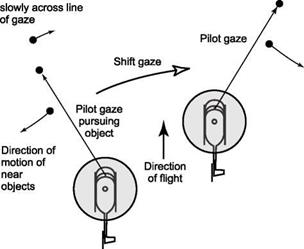
The goal of a pilotage augmentation system, designed to extend operational capability in a DVE, must be to achieve performance without compromising safety, reducing fatigue by reducing cognitive workload and increasing confidence to allow aggressive manoeuvring. The designers of such synthetic vision systems can utilize the natural, reflexive pilot skills, and several pathway-in-the-sky type formats are currently under development or being explored in research (e. g., Refs 8.34, 8.35) that exhibit such properties. Designers also have the freedom to combine such formats with more detailed display structures for precision tracking, e. g., the pad-capture mode on the AH-64A (Ref. 8.36). This type of format requires the pilot to apply cognitive attention, closing the control loop using detailed individual features to achieve the desired precision, hence risking a loss of situation awareness with respect to the outside world. Achieving a balance between precision and situation awareness is the pilot’s task and what is appropriate will change with different circumstances. Quite generally however, when equipped with an adequate sensor suite, there seems no good reason why a large part of the stabilization and tracking tasks should not be accomplished by the automatic flight control system.
Improving flying qualities for flight in a DVE is about the integration of vision and control augmentation. The UCE describes the utility and adequacy of visual cues for guidance and stabilization. The pilot rates the visual cues based on how aggressively and precisely corrections to attitude and velocity can be made. An assumption in this approach is that the aircraft has Level 1, rate command handling qualities in a GVE. In a DVE, the handling qualities of the aircraft degrade because of the impoverishment
|
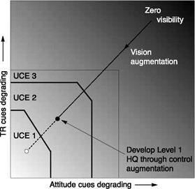
Fig. 8.36 Conceptualization of flying qualities improvements in the DVE |
of the visual cues. According to the UCE methodology of ADS-33, provided the DVE is no worse than UCE = 3, Level 1 handling qualities can be ‘recovered’ by control augmentation. The augmentation process therefore appears straightforward, at least in principle: recover to UCE = 3 or better via vision augmentation, and then use control augmentation, to recover Level 1 flying qualities – Fig. 8.36 conceptualizes this idea.
Helicopter flight in degraded visibility will remain dangerous, with a consequent higher risk to flight safety, without vision augmentation. A key characteristic of a good vision aid is that it should provide the pilot with clear and coherent cues for judging operationally relevant, desired and adequate performance standards for flight path and attitude control. The ADS-33 handling qualities requirements then provide the design criteria for control augmentation. The higher the levels of augmentation and the stronger the control feedback gains, required an increased level of safety monitoring and redundancy to protect against the negative effects of failure, which leads us to the second topic in this chapter.
As a pilot approaches rising ground, the point at which the climb is initiated depends on the forward speed and also the dynamic characteristics of the aircraft, reflected in the vertical performance capability and the time constant in response to collective pitch inputs; at speeds below minimum power, height control is exercised almost solely through collective inputs. A matched manoeuvre could be postulated as one
where the pilot applies the required amount of collective at the last possible moment so that the climb rate reaches steady state, with the aircraft flying parallel to the surface of the hill. For low-speed flight, vertical manoeuvres can be approximately described by a first-order differential equation (see Chapter 5, eqn 5.52), with its solution to a step input in the pilot’s collective lever given by
![]() w – Zww = Z9o0o w = wss(1 – eZwt)
w – Zww = Z9o0o w = wss(1 – eZwt)
In the usual notation, w is the aircraft normal velocity (positive down), wss the steady state value of w and 9o is the collective pitch angle. Zw is the heave damping derivative (see Chapter 4), or the negative inverse of the aircraft time constant in the heave axis, tw. Writing Sw = w, the time to achieve Sw can be written in the form
^ = – loge(1 – Sw) (8.33)
tw
When Sw = 0.63, t$w = tw, the heave time constant. To reach 90% of the final steady state would take 2.3 time constants and to reach 99% would take nearly 5 time constants. In ADS-33, Level 1 handling qualities are achieved if tw < 5 s, and for many aircraft types, values of 3-4 s are typical. In reality, because of the exponential nature of the response, the aircraft never reaches the steady-state climb following a step input. In fact, following a step collective, the aircraft approaches its steady-state in a particular manner. The instantaneous time to reach steady-state rate of climb – w, Tw, varies with time and is defined as the ratio of the instantaneous differential (negative) velocity to the acceleration; hence
w = – wss ZweZwt
w – wss 1 ^ (8.34)
Tw = ; = = tw
w Zw
The instantaneous time to reach steady state, Tw, is therefore a constant and equal to the negative of the time constant of the aircraft tw – a somewhat novel interpretation of the heave time constant. The step input requires no compensatory workload but, theoretically, the aircraft never reaches its destination. To achieve the steady-state goal, the pilot needs to adopt a more complex control strategy and will use the available visual cues to ensure that т w reaches zero when the aircraft has reached the appropriate climb rate; the complexity of this strategy determines the pilot workload.
In the simulation trial reported in Ref. 8.33, the pilot was launched in a low hover and requested to accelerate forward and climb to a level flight trim condition that he or she considered suited the environment. To ensure that all the visual information for stabilization and guidance was derived from the outside world, head-down instruments were turned off. After establishing the trim condition, the pilot was required to negotiate a hill with 5° slope rising 60 m above the terrain. The terrain was textured with a rich, relatively unstructured surface, and to explore the effects of degraded visual conditions fog was located at distances of 80, 240,480 and 720 m ahead of the aircraft. The fog was simulated as a shell of abrupt obscuration surrounding a sphere of ‘clear air’ centred on the pilot.
The visual cue ratings (VCRs) and associated UCEs and handling qualities ratings (HQRs) for the different cases are given in Table 8.1. The methodology adopted was an adaptation of that in ADS-33, where the UCE is derived from VCRs given by three pilots flying a set of low-speed manoeuvres. The concept of UCE >3 is also an adaptation to reflect visual conditions where the pilot was not prepared to award a VCR within the defined scale (1-5). The VCRs are also plotted on the UCE chart in Fig. 8.24. As expected, the increased workload in the DVE led the pilot to award poorer HQRs, and the UCE degraded from 1 to 3. For the HQRs, the adequate performance boundary was set at 50% of nominal height and the desired boundary at 25% of nominal height. No numerical constraints were placed on speed but the pilot was requested to maintain a reasonably constant speed.
Key questions addressed in Ref. 8.33 were ‘would the pilot elect to fly at different heights and speeds in the different conditions,’ and ‘how would these relate to the body-scaled measure, the eye-height?’ Would the pilot use intrinsic тguides to successfully transition into the climb, and what form would these take? Could the pilot control strategy be modelled based on т following principles? Earlier in this chapter we discussed a pilot’s ability to pick up visual information from the surface over which
|
Table 8.2 Average flight parameters for the terrain-hugging manoeuvres
|
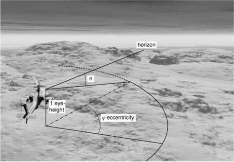
the aircraft was flying and drew attention to Ref. 8.15, where Perrone had hypothesized that the looming of patterns on a rough surface would become detectable at about 16 eye-heights (xe) ahead of the aircraft. In the various simulation exercises conducted at Liverpool there is some evidence that this reduces to about 12xe for the textured surfaces used; hence, we reference results to this metric in the following discussion.
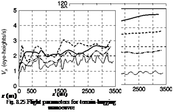
The average distances and times to the fog-lines, along with the velocity and time to the 12 eye-height point ahead of the aircraft, are given in Table 8.2. The results indicate that as the distance to the fog-line reduces the pilot flies lower and slower, while maintaining eye-height speed relatively constant. Comparing the 720-m fog-line case with the 240-m case, the average eye-height velocity is almost identical, while the actual speed and height has almost doubled. For the UCE = 3 case, the aircraft has slowed to below 2 xe per second, as the distance to the fog-line has reduced to within 20% of the 12 eye-height point. It is worth noting that the test pilot, who has extensive military and civil piloting experience, declared that the UCE = 3 case would not be acceptable unless urgent operational requirements prevailed; it simply would not be safe in an undulating, cluttered environment, and where the navigational demands would strongly interfere with guidance.
Figure 8.25 shows the vertical flight path (height in metres) and flight velocity (in metres/second and xe per second) plotted against range (metres) for the different fog cases. The pilots were requested to fly along the top of the hill for a further 2000 m to complete the run.
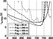
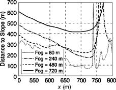
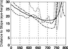
The distances along the flight path to the terrain surface, as the sloping ground is approached, are shown in Fig. 8.26. While the actual distances vary significantly, the distances in eye-heights to the surface reduce to between 12 and 16 eye-heights, as the hill is approached and during the initial climb phase. The times to contact the terrain, tsurface, are shown in Fig. 8.27. Typically, the pilot allowed rsulface to reduce to between 6 and 8 s before initiating the climb. These results are consistent with those derived in the acceleration-deceleration manoeuvre. In the UCE = 3 case (fog at 80 m) the pilot is flying at 10 m/s, giving about 8 s look-ahead time to the fog-line and only 2-3 s margin from the 12 xe point. The results suggest a relationship between the UCE and the margin between the postulated, 12 xe, look-ahead point and any obscuration; this point will be revisited towards the end of this section, but prior to this the variation of flight path angle during the climb will be analyzed to investigate the degree of t guide following during the manoeuvre.
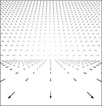
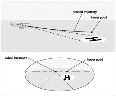
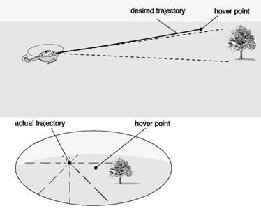
General t theory hypothesizes that the closure of any motion gap is guided by sensing and adjusting the t of the associated physical gap (Ref. 8.24). The theory reinforces the evidence presented in the previous section that information solely about Tx is sufficient to enable the gap x to be closed in a controlled manner, as when making a gentle landing or coming to hover next to an obstacle. According to the theory, and contrary to what might be expected, information about the distance to the landing surface or about the speed and deceleration of approach is not necessary for precise control of the approach and landing. The theory further suggests that a pilot might perceive t of a motion gap by virtue of its proportionality to the t of a gap in a ‘sensory flow-field’ within the visual perception system. In helicopter flight dynamics, the example of decelerating a helicopter to hover over a landing point on the ground serves to illustrate the point. The t of the gap in the optic flow-field between the image of the landing point and the centre of optical outflow (which specifies the instantaneous direction of travel, see Fig. 8.4) is equal to the t of the motion gap between the pilot and the vertical plane through the landing point. This is always so, despite the actual sizes of the optical and motion gaps being quite different; the same applies to stopping at a point adjacent to an obstacle – see Fig. 8.20.
Often movements have to be rapidly coordinated, as when simultaneously making a turn and decelerating to stop, or descending and stopping, or performing a bob-up
|
|
and, simultaneously, a 90° turn. This requires accurate synchronizing and sequencing of the closure of different gaps. To achieve this, visual cues have to be picked up rapidly and continuously and used to guide the action. т theory shows how such closed-loop control might be accomplished by keeping the т ’s of gaps in constant ratio during the movement, i. e., by т-coupling. Evidence of т-coupling in nature is presented in Refs 8.27 and 8.28 for experiments with echo-locating bats landing on a perch and infants feeding. In the present context, if a helicopter pilot, descending (along z) and decelerating (along x ), follows the т – coupling law
тл = ^z (8.16)
then the desired height will automatically be attained just as the aircraft comes to a stop at the landing pad. The kinematics of the motion can be regulated by appropriate choice of the value of the coupling constant k. There is evidence that such coupling can be exploited successfully in vision aids. For example, the system reported in Ref. 8.22 functioned on the principle of the matching of a cluster of forward-directed light beams with different look-ahead distances, which translated into times at a given speed. Such a system was designed as an aid in situations where the natural optical flow was obscured.
In many manoeuvres such as a hover turn or bob-up, there is essentially only one gap to be closed, yet the feedback actions must in principle be similar, whether there are two coupled motion gaps or just one. When a pilot is able to perceive the motion gaps associated with both the displacement and velocity, then т-coupling takes a special form,
with
Tx = k тх (8.18)
Combining eqns 8.17 and 8.18, we can write
Tx = 1 – ^ = 1 – k (8.19)
x2
Hence, the т constant strategy can be expressed as the pilot maintaining the т ’s of the displacement and velocity in a constant ratio. The more general hypothesis is that the closure of a single motion gap is controlled by keeping the т of the motion gap coupled onto what has been described as an intrinsically generated т guide, Tg (Ref. 8.24). One form of such a guide is a constant deceleration motion, from an initial condition xgo(<0), Vgo (>0) given by (c < 0)
c 2
ag = c, vg = vg0 + ct, xg = xg0 + vg01 +-12 (8.20)
At t = T, the manoeuvre duration, we can write
Substitution into the kinematic relationships in eqn 8.20 results in
The constant deceleration т guide has a T = 0.5, a result obtained earlier in this section, and coupling onto this guide with coupling constant к implies
For motions that start at rest, Vg = 0, and end at rest, we need to find a different form of guide. In Ref. 8.24, Lee argues that for natural motions such as reaching, which involve simple phases of acceleration followed by deceleration, it is reasonable to hypothesize that a simple form of intrinsic т guide will have evolved that is adequate for guiding such fundamental movements. In the context of helicopter NoE flight, any of the classic hover-to-hover repositioning manoeuvres fit into this category of motions. Indeed, in any manoeuvre that takes the aircraft from one state to another, the pilot is, in essence, closing a gap of one kind or another. The hypothesized intrinsic tau guide corresponds to a time-varying quantity, perhaps a triggered pattern within the perception system, which changes from one state to another with a constant acceleration. Surprisingly, coupling onto this ‘constant acceleration’ intrinsic guide does not, however, generate a motion of constant acceleration. The resultant motion is, rather, one with an accelerating phase followed by a decelerating phase. From a similar analyses to the case of the constant deceleration guide, the equations describing the changing Tg can be derived and written in the form
where T is the duration of the aircraft or body movement and t is the time from the start of the movement. Coupling the т of a motion gap, Tx, onto such an intrinsic tauguide, Tg, is then described by the equation
Tx = kTg (8.25)
for some coupling constant k. The intrinsic tau guide, Tg, has a single adjustable parameter, T, i. e., its duration. The value of T is assumed to be set to fit the movement either into a defined temporal structure, as when coming to a stop in a confined space, or in a relatively free way, as in the simple movement of reaching for an object. In the case of a helicopter flying from hover to hover across a clearing, we can hypothesize that time constraints are mission related and the pilot can adjust the urgency, within limits, through the level of aggressiveness applied to the controls. The kinematics of a movement can be regulated by setting both T and the coupling constant, к in eqn 8.18, to appropriate values. For example, the higher the value of k, the longer will be the acceleration period of the movement, the shorter the deceleration period and the more abruptly will the movement end. We describe situations with к values >0.5 as hard stops (i. e., к close to unity corresponds to a situation where the peak velocity is pushed close to the end of the manoeuvre) and situations with к < 0.5 as soft stops, similar to the constant T strategy.
The following of a constant acceleration guide in an accel-decel manoeuvre is conceptualized in Fig. 8.21. Both aircraft and guide, shown as a ball, start at the same
|
|
|
|
|
|
|
|
|
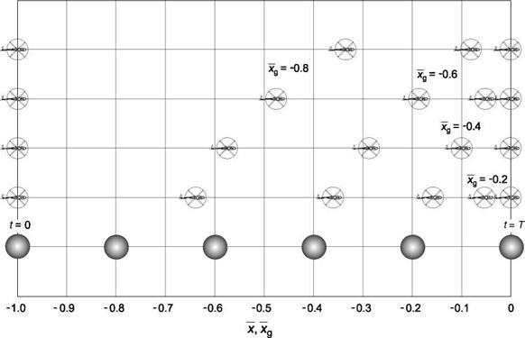
point (normalized distance Xg = —1.0) and time (t = 0) and reach the end of the manoeuvre at the same time, t = T. The ball is continuing to accelerate at this point of course, while the helicopter has come to the hover. For the case к = 0.5, the aircraft has covered about 35% of the manoeuvre distance when Xg = —0.8 and about 85% of the distance when Xg = —0.4. With к = 0.2, when Xg = —0.8, the aircraft has covered two-thirds of the manoeuvre and when Xg = —0.6, the aircraft is within 10% of the stopping point. As к increases, so does the point in the manoeuvre when the reversal from acceleration to deceleration occurs. The time in the manoeuvre when the reversal occurs, tr, can be derived as a function of the coupling coefficient к by noting that, at this point, tx = 1; from eqns 8.24 and 8.25, we can write
"=2 (■+(2)1=1 (826)
This equation can be rearranged into the form
tr=22—yT (827)
Thus, when к = 0.2, tr = 0.333T, when к = 0.4, tr = 0.5T and when к = 0.6, tr = 0.67T, etc.
When two variables, i. e., the motion x and the motion guide Xg, are related through their t-coupling in the form of eqn 8.25, it can be shown (Ref. 8.23) that they are also related through a power law
x a x]Jк (8.28)
This relationship is ubiquitous in nature, governing the relationships between stimuli and sensory responses. Normalizing the distance and time by the manoeuvre length and duration respectively, the motion kinematics (for negative initial x) can be written
as
The coupling parameter к determines exactly how the closed-loop control functions, e. g., proportional as к approaches 1 or according to a square law when к = 0.5. The manoeuvre kinematics are presented in Fig. 8.22 of a motion that perfectly tracks the constant acceleration t guide for various values of coupling constant к. The motion t is shown in Fig. 8.22(a), the motion gap, X, in Fig. 8.22(b), the gap closure rate (normalized velocity) in Fig. 8.22(c) and the normalized acceleration in Fig. 8.22(d); all are shown plotted against normalized time.
The closure rate, shown in Fig. 8.22(c), illustrates a typical accel-decel-type velocity profile (cf. X in Fig. 8.16). For к = 0.2 the maximum velocity occurs about 30% into the manoeuvre, while for к = 0. 8 the peak occurs close to the end of the
manoeuvre.
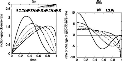 |
Fig. 8.22 Profiles of motions following the constant acceleration guide
An example of the success of this more general strategy is shown in Fig. 8.23, showing the same case from Ref. 8.31, illustrated previously in Fig. 8.16, but now for the helicopter flying the complete accel-decel manoeuvre. The coupling coefficient is 0.28, giving a power factor of 3.5, with a correlation coefficient of 0.98.
In the analysis of the Ref. 8.31 data, the start and end of the manoeuvres were cropped at 10% of the peak velocity. The tests were flown on the DERA/QinetiQ large motion simulator as part of a series of tests with a Lynx-like helicopter examining the effect of levels of aggressiveness on handling qualities and simulation fidelity. Considering all 15 accel-decels that were flown, the mean values of k follow the trends expected based on Fig. 8.22 (low aggression, k = 0.381; moderate aggression, k = 0.324; high aggression, k = 0.317). As the aggression level increases, the pilot elects to initiate the deceleration earlier in the manoeuvre: low aggression 0.5T into manoeuvre when т ~ 6 s; high aggression 0.4T into manoeuvre when т ~ 4.5 s. The pilot is more constrained during the deceleration phase, with the pilot limiting the nose-up attitude to about 20° to avoid a complete loss of visual cues in the vertical field of view.
0
![]()
![]()
![]()
![]()
![]()
![]()
![]()
![]()
![]()
![]()
 -60
-60
An intrinsic t guide is effectively a mental model, created by the nervous system, which directs the motion. It clearly has to be well informed (by visual cues in the present case) to be safe. Constant acceleration is one of the few natural motions, created in the short term by the gravitational field, so it is not surprising that the perception system might well have developed to exploit such motions. But the nature of the coupling, the chosen manoeuvre time T and profile parameter к must depend on the performance capability of the aircraft (or the animal performing a purposeful action), and pilots (or birds) need to train to ‘programme’ these patterns into their repertoire of flying skills. When the visual environment degrades so does the ability of the pilot’s perception system to pick up the required information and hence to track the error between actual motions and intrinsic guides. The UCE is, in a sense, a measure of this ability, suggesting that there should be a relationship between UCE and the t of the motion when initiating a manoeuvre to stop, turn or pull-up. In the low-aggression case of Ref. 8.31, the pilot returned Level 1 HQRs and initiated the deceleration when t ~ 6 s, taking about 10 s to come to the hover. The pilot could clearly pick up the visual ‘cues’ of the trees at the stopping point throughout.
The question of how far, or more appropriately how long, into the future the pilot needs to be able to see is critical to flight safety and the design of vision augmentation systems. The research reported in Ref. 8.31 has been extended to address this question specifically, and preliminary results are reported in Ref. 8.33. The focus of attention in this study was terrain following in the presence of degraded visibility, in particular fog, and we continue this chapter with a review of the results of this work and analysis of low-speed terrain following in the DVE.
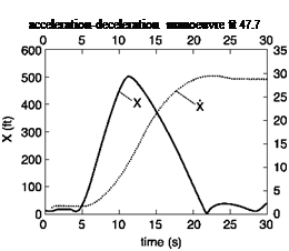 |
Figure 8.15 shows a schematic of an acceleration-deceleration manoeuvre, showing the distance to go to stop at x = 0. Figure 8.16 shows the kinematic profile of a helicopter
Fig. 8.16 Kinematics of the acceleration-deceleration manoeuvre
time (s)
 |
flying a 500 ft accel-decel in a flight simulator trial, and Fig. 8.17 shows the variation of time to stop, Tx, during the deceleration phase of the manoeuvre. The data are taken from Ref. 8.31, where the author and his colleagues introduced the concept of т – control in helicopter flight, also described as prospective control in recognition of the temporal nature of flight control. The deceleration is seen to extend from about 11 s into the manoeuvre, when the peak velocity is about 30 knots, for about 10 s, when the time to stop is nearly 6 s.
Figure 8.17 shows that the correlation of тх with time is very strong, with a correlation coefficient R2 of 0.998. The slope of the fit, i. e., T, is 0.58, indicating a non-constant deceleration with peak during the second half of the manoeuvre. So the pilot initiates the deceleration when the time to stop is about 6 s and holds an approximately constant T strategy through to the stop.
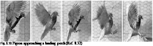
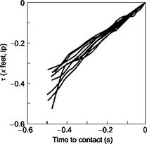
As referred to above, the use of т in motion control has been the subject of research in the natural world for some time. In Ref. 8.32, Lee and colleagues have measured the т control strategy of pigeons approaching a perch to land. Figure 8.18 shows a sequence of stills taken during the final 0.5 s of the manoeuvre. The analysis of the photographic data shows that the pigeon controls braking in the last few moments of flight by maintaining a constant T for the gap between its feet and the perch, as shown in Fig. 8.19. The т of the pigeon’s feet to the landing position is given by т(Xfeet, Ip). The feet are moving forward and the head is moving back, so the visual ‘cues’ are far from simple. The average slope of the lines in Fig. 8.19 (т) is about 0.8, indicating that
|
Fig. 8.19 Time to land for pigeon approaching a perch (Ref. 8.32) |
the maximum braking occurs very late in the manoeuvre – the pigeon almost crash lands, or at least experiences a hard touchdown, which ensures positive contact and is probably quite deliberate.
So how does a pilot or a pigeon manage to maintain a constant T, or indeed any other t variation, as they approach a goal? In addressing this question for action in the natural world, Lee gives a new interpretation to the whole process of motion control, which has significant implications for helicopter flight control and the design of augmentation systems. We now turn to the general theory of t-coupling, which also addresses the need for controlling several motion t ’s in more complex manoeuvres and introduces the concept of the motion guide and its associated t.
When xe >> 1 (or x >> z), we can simplify eqns 8.1 and 8.3 to the form
![]() (8.5)
(8.5)
The ratio of distance to velocity is the instantaneous time to reach the viewpoint, which we designate as т (t),
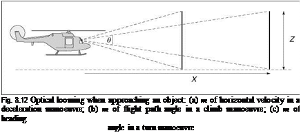
This temporal optical variable is considered to be important in flight control. A clear requirement for pilots to maintain safe flight is that they are able to predict the future trajectory of their aircraft far enough ahead so that they can stop, turn or climb to avoid a hazard or follow a required track. This requirement can be interpreted in terms of the pilot’s ability to detect motion ahead of the aircraft. In his explorations of temporal optical variables in nature (Refs 8.23-8.28), David Lee makes the fundamental point that an animal’s ability to determine the time to pass or contact an obstacle or piece of ground does not depend on explicit knowledge of the size of the obstacle, its distance away or relative velocity. The ratio of the size to rate of growth of the image of an obstacle on the pilot’s retina is equal to the ratio of distance to rate of closure, as conceptualized in Fig. 8.12, and given in angular form by eqn 8.7.
 |
apply computations on the more primitive variables of distance or speed, thus avoiding the associated lags and noise contamination. The time-to-contact information can readily be body scaled in terms of eye-heights, using a combination of surface and obstacle т (t)’s, thus affording animals with knowledge of, for example, obstacle heights relative to themselves.
While making these assertions, it is recognized that much spatial information is available to a pilot and will provide critical cues to position and orientation and perhaps even motion. For example, familiar objects clearly provide a scale reference and can guide a pilot’s judgement about clearances or manoeuvre options. However, the temporal view of motion perception purports that the spatial information is not essential to the primitive, instinctive processes involved in the control of motion.
Tau research has led to an improved understanding of how animals and humans control their motion and humans control vehicles. A particular interest is how a driver or pilot might use т to avoid a crash state, or how т might help animals alight on objects. A driver approaching an obstacle needs to apply a braking (deceleration) strategy that will avoid collision. One collision-avoid strategy is to control directly the rate of change of optical tau, which can be written in terms of the instantaneous distance to stop (x), velocity (x) and acceleration (x) in the form:
xx
т = 1 – -^ (8.8)
x2
The system used here for defining the kinematics of motion is based on a negative gap x being closed. Hence, with x < 0 and x > 0, т > 1 implies accelerating flight, т = 1 implies constant velocity and т<1 corresponds to deceleration. In the special case of a constant deceleration, the stopping distance from a velocity x is given by
Hence, a decelerating helicopter will stop short of the intended hover point if at any point in the manoeuvre
![]() -x2
-x2
2x
Using eqns 8.7 and 8.8, this condition can be written more concisely as
dr
— < 0.5 (8.11)
dt
A constant deceleration results in Г progressively decreasing with time and the pilot stopping short of the obstacle, unless Г = 0.5 when the pilotjust reaches the destination.
The hypothesis that optical r and Г are the variables that evolution has provided the animal world with to detect and rapidly process visual information, suggests that these should be key variables in flight guidance. In Ref. 8.26, Lee extends the concept to the control of rotations, related to how athletes ensure that they land on their feet after a somersault. For helicopter manoeuvring, this can be applied to control in turns, connecting with the heading component of flight motion, or in vertical manoeuvres, with the flight path angle component of the motion. For example, with heading angle ф and turn rate ф, we can write angular r as
ф
r (t) = у (8.12)
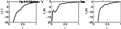
A combination of angular and translational r ’s, associated with physical gaps, needs to be successfully picked up by pilots to ensure flight safety. Figure 8.13 illustrates three examples of motion r variations as a function of normalized manoeuvre time. The results are derived from flight simulation tests undertaken on the Liverpool Flight Simulator in, nominally, good visual conditions. In all three cases the final stages of the manoeuvre (t approaches 1) are characterized by a roughly constant Г, implying, as noted above, a constant deceleration to the goal.
Reaching a goal with a constant Г can be achieved without a constant deceleration of course, and we shall see later in this chapter what the different deceleration profiles look like. For example, if the maximum deceleration towards the goal occurs late in the manoeuvre, then 0.5 <T < 1.0, while an earlier peak deceleration corresponds to 0.0 < Г < 0.5. An interesting case occurs when Г = 0, so that however close to the goal r remains a constant c, i. e.,
x
r = – = c (8.13)
x
The only motion that satisfies this relationship is an exponential one, with the goal approached asymptotically.
An interesting discovery of r control, although unbeknown at the time, is described in Ref. 8.29. In the early 1970s, researchers at NASA Langley conducted flight
0
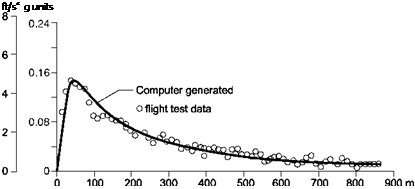 |
400 800 1200 1600 2000 2400 2800 ft
1 l___________ l___________ l___________ l___________ l____________ l___________ l
Range
Fig. 8.14 Deceleration profile for helicopter descending to a landing pad (from Ref. 8.29)
trials using several different helicopter types in support of the development of instrument flight procedures and the design of flight director displays to aid pilots during the approach and landing phases in poor visibility conditions. The engineers had postulated particular deceleration profiles as functions of height and distance from the landing zone, and the pilots were asked to evaluate the systems based on workload and performance. Several different design philosophies were evaluated and the pilots commented that none felt intuitive and that they would use different control strategies in manual landings, particularly during the final stages of the approach. The linear deceleration profiles resulted in pilots concerned that they were being commanded to hover well short of the touchdown point. The constant deceleration profile was equally undesirable and led to a high pitch/low power condition as the hover was approached. The pilots were asked to fly the approaches manually in good visual conditions, from which the deceleration profiles would be derived and then used to drive the flight director. Figure 8.14 shows a typical variation of deceleration during the approach with 50 knots initial velocity at 500 ft above the ground.
Also shown in the figure is the computer-generated profile showing a gradual reduction in speed until the peak deceleration of about 0.15 g is reached 70 m from the landing pad. The ‘computer-generated’ relationship between acceleration, velocity and distance took the form
where k is a constant derived from the initial conditions. Recalling the formulae for т in eqn 8.8, the relationship given by eqn 8.14 can be written in the form
1 – t = kx1-n (8.15)
The parameters k and n were computed as constants in any single deceleration but varied with initial condition and across the different pilots. The range power parameter
n varied between 1.2 and 1.7. Note that a value of unity corresponds to a constant t for the whole manoeuvre. Equation 8.15 suggests that, at long range, the pilot is maintaining constant velocity (t=1), consistent, of course, with the steady initial flight
і
condition. As range is reduced, т reduces until x = kn-1 when т = 0 and the approach becomes exponential. Beyond this, the representation in eqn 8.15 breaks down, as it predicts a negative т, i. e., the helicopter backs away from the landing pad, although this can happen in practice. Approaches at constant т may seem ineffective because the goal is never reached, but there is evidence that pilots sometimes use this strategy during the landing flare in fixed-wing aircraft, perhaps as a ‘holding’ strategy as the flight path lines up with the desired trajectory (see Ref. 8.30).
The concept of t in motion control has significance for helicopter flight in degraded visual conditions. If the critical issue for sufficiency of visual cues is that they afford the information to allow the pilot to pick up т ’s of objects and surfaces, then it follows that the т ’s are measures of spatial awareness. It would also follow that they would be appropriate measures to use to judge the quality of artificial vision aids and form the underlying basis for the design and the information content of vision aids. This author has conducted a number of experiments to address the question – how do pilots know when to stop, or to turn or pull up to avoid collision? In the following sections some results from this research will be presented.
One of the earliest published works on visual perception in flight control presented a mathematical analysis of ‘motion perspective’ as used by pilots when landing aircraft (Ref. 8.11). The first author of this work, James Gibson, introduced the concept of the optical flow and the centre of expansion when considering locomotion relative to, and particularly approaching, a surface. Gibson suggested that the ‘psychology of aircraft landing does not consist of the classical problems of space perception and the cues to depth’. In making this suggestion, Gibson was challenging conventional wisdom that piloting ability was determined by the sufficiency of linear/aerial perspective and parallax cues. Gibson had earlier introduced the concept of motion perspective in Ref. 8.12, but in applying it to flight control he laid the foundation for a new understanding of, what we might generally call, spatial awareness. To quote from Ref. 8.11:
Speaking in terms of visual sensations, there might be said to exist two distinct characteristics of flow in the visual field, one being the gradients of ‘amount’ of flow and the other being the radial patterns of ‘directions’ of flow. The former may be considered a cue for the perception ofdistance and the latter a cue for the perception of direction of locomotion relative to the surface.
Gibson focused mainly on fixed-wing landings but he also presented an example of the optical flow-field generated by motion perspective for the case of a helicopter landing vertically, as shown in Fig. 8.3. ‘For the case of a helicopter landing, the apparent
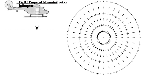
velocity of points in the plane below first increases to a maximum and then decreases again.’ The optical flow-field concept clearly has relevance to a helicopter landing at a heliport, on a moving deck or in a clearing, and raises questions as to how pilots reconstruct a sufficiently coherent motion picture from within the confines of a closed – in cockpit to allow efficient use of such cues.
Gibson’s ecological approach (Ref. 8.13) is a ‘direct’ theory of visual perception, in contrast with the ‘indirect’ theories which deal more with the reconstruction and organization of components in the visual scene by the visual system and associated mental processes (Ref. 8.14). The direct theory can be related to the engineering theory of handling qualities. The flight variables of interest when flying close to obstacles and the surface are encapsulated in the definition of performance requirements in the ADS – 33 flight manoeuvres – speed, heading, height above surface, flight path accuracies, etc. In visual perception parlance these have been described as ego-motion attributes (Ref. 8.14) and key questions concern the relationship between these and the optical variables, like Gibson’s motion perspective. If the relationships are not one-to-one then there is a risk of uncertainty when controlling the ego motion. Also, are the relationships consistent and hence predictable? The framework for the discussion is a set of three optical variables considered critical to recovering a safe UCE for helicopter nap-of-the – earth (NoE) flight – optical flow, differential motion parallax and the temporal variable tau, the time to contact or close a gap.
Figure 8.4, from Ref. 8.15 (contained within Ref. 8.16), illustrates the optical flow-field when flying over a surface at 3 eye-heights per second (corresponds to fast NoE flight – about 50 knots at 30-ft height – or the flow-field observed by a running person). The eye-height scale has been used in human sciences because of its value to deriving body-scaled information about the environment during motion. Each flow vector represents the angular change of a point on the ground during a 0.25-s snapshot. Inter-point distance is 1 eye-height. The scene is shown for a limited field-of-view
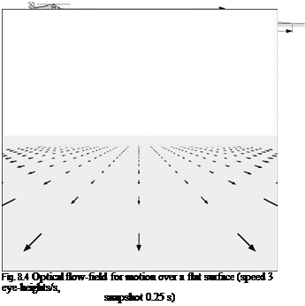 |
window, typical of current helmet-mounted display formats. A 360° perspective would show flow vectors curving around the sides and to the rear of the aircraft (see Gibson, Ref. 8.12). The centre of optical expansion is on the horizon, although the flow vectors are shown to ‘disappear’ well before that, to indicate the consequent ‘disappearance’ of motion information to an observer with normal eyesight. If the pilot were to descend, the centre of optical expansion would move closer to the aircraft, in theory giving the pilot a cue that his or her flight trajectory has changed.
The length of the flow vectors gives an indication of the motion cues available to a pilot; they appear to decrease rapidly with distance. In the figure, the ‘flow’ is shown to disappear after 16 eye-heights.
The velocity in eye-heights per second is given by
In terms of the optical flow, or rate of change of elevation angle 9 (Fig. 8.5), we can write
![]() d9 X. e
d9 X. e
dt 1 + x2
where xe is the pilot’s viewpoint distance ahead of the aircraft scaled in eye-heights.
|
When the eye-height velocity, xe, is constant, then the optical flow is also constant; they are in effect measures of the same quantity. However, the simple linear relationship between xe and ground speed given by eqn 8.2 is disrupted by changes in altitude. If the pilot descends while keeping forward speed constant, xe increases; if he climbs, xe decreases. A similar effect is brought about by changes in surface layout, e. g., if the ground ahead of the aircraft rises or falls away. Generalizing eqn 8.2 to the case where the aircraft has a climb or descent rate (djz) relative to the ground, we obtain
The relationship between optical flow rate and the motion variables is no longer straightforward. Flow rate and ground speed are uniquely linked only when flying at constant altitude.
A related optical variable comes in the form of a discrete version of that given by eqn 8.2 and occurs when optically specified edges within the surface texture pass some reference in the pilot’s field of vision, e. g., the cockpit frame usually serves as such a reference. This optical edge rate is defined as
|
Fig. 8.6 Angular velocity versus distance along ground plane (Ref. 8.15) |
optical flow rate, edge rate is invariant as altitude changes. However, when ground speed is constant, edge rate increases as the edges in the ground texture become denser, and decreases as they becomes sparser.
From eqn 8.2, it can be seen that flow rate falls off as the square of the distance from the observer. Figure 8.6, from Ref. 8.15, shows how the velocity, in minutes-of – arc/second, varies with distance for an eye-point moving at 3 eye-heights/s.
Perrone suggests that a realistic value for the threshold of velocity perception in complex situations would be about 40 min arc/s. In Fig. 8.6, this corresponds to information being subthreshold at about 15-16 eye-heights distant from the observer. To quote from Ref. 8.15, ‘This is the length of the “headlight beam” defined by motion information alone. At a speed of 3 eye-heights/sec, this only gives about 5 seconds to respond to features on the ground that are revealed by the motion process’. The value of optical streaming for the detection and control of speed and altitude has been discussed in a series of papers by Johnson and co-workers (Refs 8.16-8.20). Flow rate and texture/edge rate are identified as primary cues. These velocity cues can be picked up from both foveal (information detected by the central retinal fovea) and ambient (information detected by the peripheral retina) vision. An issue with ambient information, however, is the significant degradation in visual acuity as a function of eccentricity. The fovea of the human eye, where there is a massive concentration of visual sensors, has a field of regard of less than 1° (approximately a thumb’s width at arm’s length). The visual acuity at 20° eccentricity is about 15% as good as the fovea for resolution, although Cutting points out that this increases to 30% for motion detection (Ref. 8.21). Cutting also observes that the product of motion sensitivity and motion flow (magnitude of flow vectors) when moving over a surface is such that ‘the thresholds for detecting motion resulting from linear movement over a plane are roughly the same across a horizontal meridian of the retina’.
In Fig. 8.4, the centre of optical expansion or outflow is on the horizon. If the pilot is looking directly at this point then the information seen will be ‘filtered’ by the
0 10 20 30 40 50
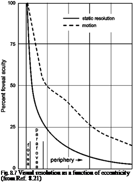 |
Degrees eccentricity ip
variable sensitivity across the retina. The motion acuity gradient or visual resolution takes the form illustrated in Fig. 8.7 (Ref. 8.21), based on the eccentricity and elevation angles defined in Fig. 8.5.
In Fig. 8.7, data are shown for static resolution and motion resolution referenced to the fovea performance of 100. The results show that the strength of visual inputs 20° off-centre reduce to about 40% of those picked up by the fovea when in motion compared with 15% statically. However, the magnitude of the motion flow vectors depicted in Fig. 8.4 increases away from the line of sight in a normalized manner shown in Fig. 8.8 (also from Ref. 8.21). The sensitivity of the retina to motion is therefore the resultant product of the two effects and is actually fairly uniform across a horizontal meridian. Figure 8.9 shows the case for viewing at 8° below the horizon, corresponding to about 7 eye-heights ahead of the aircraft.
A more irregular surface will give rise to deformations in the sensitivity but the same underlying effect will be present, leading to the conjecture that the pilot’s gaze will naturally be drawn to the direction of flight, i. e., that direction which, on average, gives uniform stimulation across the retina. This is good news for pilots, and a determining factor on piloting skill is how well this capability is ‘programmed’ into an individual’s perceptual system.
The subject of way-finding, or establishing the direction of flight, has also been addressed in some detail in Ref. 8.21, where the notion of directed perception was introduced. Cutting developed the optical flow-field concept, arguing that people and animals make more use of the retinal flow-field, fixating with the fovea on specific
|
0 20 40 60 80
Degrees eccentricity f
|
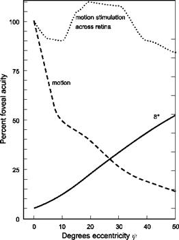
|
|
|
parts of the environment and deriving information from the way in which surrounding features move relative to that point on the retina. In this way the concept of differential motion parallax (DMP) was hypothesized as the principal optical variable used for wayfinding in a cluttered environment. Figure 8.10 illustrates how motion and direction of motion can be derived from DMP. The helicopter is being flown through a cluttered environment. The pilot fixates his or her gaze on one of the obstacles (to the left of motion heading) and observes the motion parallax effects on objects closer and farther away. Objects farther away move to the right and those closer move to the left of the gaze (as seen on the retinal array). The pilot can judge which objects are closer and further away by the relative velocities. Figure 8.10 indicates that closer objects move more quickly across the line of gaze. There is no requirement to know the actual size or distance of any of the objects in the clutter. The pilot can judge from this motion perception that the direction of motion is to the right of the fixated point. He or she can now fixate on a different object. If objects further away (slower movements) move
to the left and those closer (faster movements) move to the right, then the pilot will perceive that motion is to the left of the fixated object. By applying a series of such fixations the pilot will be able to keep updating his or her information about direction of motion, and home in on the true direction with potentially great accuracy (the point where there is no flow across the line of gaze). Cutting observed that in high – performance situations, for example, deck landings of fixed – and rotary-wing aircraft, required heading accuracies might need to be 0.5° or better. DMP does not always work however, e. g., in the direction of motion itself or in the far field, where there is no DMP, or in the near field, where DMP will fail if there are no objects nearer than half the distance to the point of gaze (Ref. 8.21).
In Ref. 8.15, Perrone also discusses the question of how pilots might infer surface layout, or the slants of surfaces, ahead of the aircraft. This is particularly relevant to flight in a DVE where controlled flight into terrain is a major hazard and still all too common. The correct perception of slope is critical for achieving ‘desired’ height safety margins for flight over undulating terrain, and hence for providing good visual cue ratings for vertical translational rate, for example. Figure 8.11 illustrates the flow- field when approaching a 60° slope hill about 8 eye-heights away. The centre of optical
|
|
|
Fig. 8.11 Optical flow-field approaching a 60° slope (from Ref. 8.15) |
expansion has now moved up the slope and the motion cues over a significant area around this are very sparse. If the pilot wants to maintain gaze at a point where the motion threshold cuts in (e. g., 5 s ahead) he or she will have to lift his or her gaze, and pilots will tend to do this as they approach a hill. This aspect is discussed again later in this chapter when results are presented from simulation research into terrain flight, where the question – how long do pilots look forward? – is addressed.
Any vision augmentation system that tries to infer slope based on flow vectors around the centre of expansion is likely be fairly ineffective. In Ref. 8.22, a novel vision augmentation system was proposed for aiding flight over featureless terrain at night. An obstacle detector system was evaluated in simulation, consisting of a set of cueing lights, each with a different look-ahead time, presenting a cluster of spots to the pilot of the light beams on the terrain ahead of the aircraft. As altitude or the terrain layout ahead changed, so the cluster changed shape, providing the pilot with an ‘intuitive spatial motion cue’ to climb or descend.
In a cluttered environment, the optical variables – flow/edge rate and DMP – appear to provide primary cues to pilots for judging the direction in which they are heading. The question as to how they judge their speed and distance takes us onto the third optical flow variable in this discussion, the results of which suggest that pilots do not actually need to know speed and distance for safe flight control; rather the prospective control is temporally based within an ordered spatial environment.