Category Management and Minimisation of Uncertainties and Errors in Numerical Aerodynamics

Modelling of Uncertainties in the Airfoil Geometry

We model uncertainties in the geometry of RAE-2822 airfoil via random boundary perturbations:

д&£(ю) = {x + £k(x, w)n(x) : x Є dG}, (5)

where n(x) is the normal vector in a point x, k(x, со) a random field, G the computa­tional geometry and є 1. We assume that the covariance function is of Gaussian type

COk(Ki, K2) = cr2-exp(-d2), d = yjxi – x2|2//2+|Zi-Z2|2//22,

Table 1 Statistics obtained for uncertainties in the airfoil geometry. We used the Gaussian covariance function, PCE of order P = 1 with M = 3 random variables and the sparse Gauss – Hermite grid with nq = 25 points.

mean

st. dev. <T

<T/mean

CL

0.8552

0.0049

0.0058

CD

0.0183

0.00012

0.0065

where к1 = k((x1,0,zi), ю), k2 = ((x2,0,z2),ffl) are two random variables in points (xi,0,z1) and (x2,0,z2). For numerical simulations we take the covariance lengths l1 = | maxi(xi) – min;(xj)|/10and l2 = | max^(zi) – mini(zi)|/10, standard deviation а = 10-3, m = 3 the number of KLE terms (see Eq. 6), the stochastic dimension M = 3 and the number of sparse Gauss-Hermite points (in 3D) for computing PCE coefficients in (Eq. 8) nq = 25. In [13] one can see 21 random realisations of RAE – 2822 airfoil.

Table 1 demonstrates the surprisingly small uncertainties (the last column) in the lift and in the drag — 0.58% and 0.65% correspondingly. A possible explanation can be small uncertain perturbations in the airfoil geometry.

Modelling of Uncertainties in Parameters

We assume that the free-stream turbulence in the atmosphere randomly and simul­taneously changes the velocity vector or, what is equivalent the Mach number Eq. 4 and the angle of attack Eq. 3. One should not mix this kind of turbulence with the turbulence in the boundary layer reasoned by friction. It is assumed that turbulence vortices in the atmosphere are comparable with the size of the airplane. The free – stream turbulence in the atmosphere is modelled by two additionally axes-parallel velocity vectors v1 := v1(91) and v2 := v2(Q2) (Fig. 1), which have Gaussian distri­bution [13]. We model the free-stream turbulence via two random vectors (in 3D it will be three vectors) vi and v2 which change a and Ma (see Fig. i):

o9i ов2

Vl = ~/2 an^ V2 = ~/2′

where 91 and 92 are two Gaussian random variables with zero mean and unit vari­ance, a := Iu„, I the mean turbulence intensity and u«, the undisturbed free stream velocity beyond the boundary layer. This mean turbulence intensity is often used for characterising turbulence in a wind tunnel. For instance, I = 0.001 means low turbulence, I = 0.002 middle and I = 0.005 high turbulence.

Denoting

9 := J9f + 9}, v := sj\ + /3 := arctg^ and г := ^L, (2)

and performing easy geometrical computations, obtain the new angle of attack and the new Mach number:

Modelling of Uncertainties in Parameters

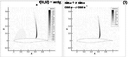
Fig. 2 (left) The difference Ap := |p — p| between the deterministic density p := p(ot, Ma) and the mean density p. (right) The same is for the pressure Ap := p — p. Here p Є (0.5,1.2) and p є (0.7,1.3).

/ J_^ і—

Ma (0i,02) = May 1 H—————- v2l0cos(/3 + a). (4)

Further we study how uncertainties in a and Ma spread into the solution. We note that uncertainties in a and in Ma can be modelled in a different way (see e. g. [23], [27]). >From the construction one can see that Ma := E(Ma (01,02)) and a := E(af (01,02)) are equal to the deterministic values Ma and a, here E(-) is the mathematical expectation. In Fig. 2 (left) we compare the deterministic dens­ity p(a, Ma) with the p := E(p(a (0i, 02),Ma (0i, 02))) for the Case 9 (a = 2.79, Ma := 0.734). In Fig. 2 (right) we do the same comparison for the deterministic pressure. One can see a large difference in the shock position. This large difference motivates us to model uncertainty in a and in Ma.

Numerical Methods for Uncertainty Quantification and Bayesian Update in Aerodynamics

Alexander Litvinenko and Hermann G. Matthies

Abstract. In this work we research the propagation of uncertainties in parameters and airfoil geometry to the solution. Typical examples of uncertain parameters are the angle of attack and the Mach number. The discretisation techniques which we used here are the Karhunen-Loeve and the polynomial chaos expansions. To integ­rate high-dimensional integrals in probabilistic space we used Monte Carlo simula­tions and collocation methods on sparse grids. To reduce storage requirement and computing time, we demonstrate an algorithm for data compression, based on a low – rank approximation of realisations of random fields. This low-rank approximation allows us an efficient postprocessing (e. g. computation of the mean value, variance, etc) with a linear complexity and with drastically reduced memory requirements. Finally, we demonstrate how to compute the Bayesian update for updating a priori probability density function of uncertain parameters. The Bayesian update is also used for incorporation of measurements into the model.

1 Introduction

Nowadays, the trend of numerical mathematics is often trying to resolve inexact mathematical models by very exact deterministic numerical methods. The reason of this inexactness is that almost each mathematical model of a real world situation contains uncertainties in the coefficients, right-hand side, boundary conditions, ini­tial data as well as in the computational geometry. All these uncertainties can affect the solution dramatically, which is, in its turn, also uncertain. The information of the interest is usually not the whole set of realisations of the solutions (too much data), but some other stochastic information: cumulative distribution function, probability density function, mean value, variance, quantiles, exceedance probability etc.

Alexander Litvinenko • Hermann G. Matthies

Institute of Scientific Computing, Technische Universitat Braunschweig, Hans-Sommer str. 65, 38106, Braunschweig, Germany e-mail: wire@tu-bs. de

http://www. wire. tu-bs. de

B. Eisfeld et al. (Eds.): Management & Minimisation of Uncert. & Errors, NNFM 122, pp. 265-282. DOI: 10.1007/978-3-642-36185-2_11 © Springer-Verlag Berlin Heidelberg 2013

During the last few years, one can see an increasing interest in numerical methods for solving stochastic computational fluid dynamic (CFD) problems [3, 8, 17, 19, 24, 26]. In this work we consider an example from aerodynamics, described by a system of Navier-Stokes equations with a k-w turbulence model. Uncertainties in parameters such as the angle of attack a and Mach number are modelled by random variables, uncertainties in the shape of the airfoil are modelled by a random field [14, 12]. Uncertain output fields such as pressure, density, velocity, turbulence kinetic energy are modelled by random fields as well. The lift, drag and moments will be random variables.

We assume that there is a solver which is able to solve the deterministic (without uncertainties) Navier-Stokes problem. In this work we used the TAU code (de­veloped in DLR) with k-w turbulence model [4]. We also assume that spatial discret­isation of the airfoil is given. Our job is the appropriate modelling of uncertainties and developing stochastic/statistical numerical techniques for further quantification of uncertainties. At the same time, due to the high complexity of the deterministic solver, we are allowed to use only non-intrusive stochastic methods such as Monte Carlo or collocation methods. So, we are interested in methods which do not require changes in the deterministic code.

The rest of the paper is structured as follows. In Section 3 we describe the prob­lem and discretisation techniques, such as the Karhunen-Loeve expansion (KLE) [16] and polynomial chaos expansion (PCE) of Wiener [25]. In Section 2.1 we ex­plain how we model uncertainties in the parameters angle of attack and Mach num­ber. Uncertainty in the airfoil geometry is described in Section 2.2. The low-rank response surface is presented in Section 4. To avoid large memory requirements and to reduce computing time, low-rank techniques for representation of input and output data (solution) were developed in Section 5. Section 7 is devoted to the nu­merical results, where we demonstrate the influence of uncertainties in the angle of attack a, in the Mach number Ma and in the airfoil geometry on the solution – drag, lift, pressure and absolute friction coefficients. The strongly reduced memory re­quirement for storage stochastic realisations of the solution is demonstrated as well. In Section 6 we demonstrate how to use the Bayesian update (BU) for improving the statistical description of the random airfoil geometry. Section 7 is devoted to other numerical experiments.

2 Statistical Modelling of Uncertainties

The problem to consider in this work is the stationary system of Navier-Stokes equa­tions with uncertain coefficients and parameters:

v(x, co) ■ Vv(.r, со) – ^V2v(.r, со) + Vp{x, со) = g(x) хє&, со e Q V • v(x, ю) = 0

u

Numerical Methods for Uncertainty Quantification and Bayesian Update in Aerodynamics

Fig. 1 Two random vectors vj and V2 model free-stream turbulence, u and u old and new free stream velocities, a and a old and new angles of attack with some initial and boundary conditions. Here v is velocity, p pressure and g the right-hand side, the computational domain G is RAE-2822 airfoil with some area around. Examples of uncertain parameters are the angle of attack a and the Mach number Ma. Uncertainty in the airfoil geometry is modelled via random field (see Section 7).

Summary and Conclusion

In the described studies CFD settings are systematically varied by using a minimum number of simulations to quantify the relative impact of several numerical and geo­metrical parameters on the CFD result. The Taguchi method is applied to reduce the number of simulations in comparison to a full parameter variation. Statistical analysis (ANOVA) gave informations about the relative parameter influence on the CFD results like lift and drag. It also gives information on interactions between dif­ferent parameters and their influence on the result. During the studies steady and unsteady test cases are performed and in both cases the results reflect long lasting experiences in CFD simulation. It is also shown that the results achieved by the

Summary and Conclusion

Fig. 12 Results of run 8. A = Reynolds number, B = Mach number, C = angle of attack

Taguchi method are robust to stronger variations of all parameters. This makes the results more generally valid, at least as long as the parameters are not varied too strongly. Therefore, the performed study shows that the Taguchi method is a suit­able systematic method to check the accuracy of CFD simulations. To reduce the effort even more the Taguchi-Method was implemented into the TAU code via Py­thon scripts. The scripts support the user during the selection of the Taguchi matrix and setup automatically all necessary TAU input files and folders.

References

[1] AR-138, Experimental Data Base for Computer Program Assessment, ch. A6-1 (1979)

[2] Klein, B.: Versuchsplanung-DOE: Einfuhrung in die Taguchi/Shainin-Methodik, 2nd edn., Oldenburg

[3] Blasing J. P. (Hrsg.): Workbook DoE, Design of Experiments nach G. Taguchi, TQU

[4] Roos, P. J.: Taguchi Techniques for Quality Engineering. 2. McGraw-Hill, Auflage

[5] Hering, Triemel, Blank: Qualitatssicherung fur Ingenieure. VDI Verlag

[6] Lutz, T., Sommerer, A., Wagner, S.: Parallel Numerical Optimisation of Adaptive Tran­sonic Airfoils. In: Fluid Mechanics and its Applications, vol. 73. Kluwer Academic Publishers

TAU Implementation

To automatize the procedure and to reduce the required effort it was decided to implement the Taguchi method into the TAU Code by using Python scripts. The new script, which was published with the TAU 2012 release supports the user dur­ing the selection of the Taguchi Matrix, its modification and in the consideration of interactions. Several parameters can be chosen from a given list, which can be extended at any time. After defining parameteres and their levels para files (TAU control file), job files (to start the simulation on the high performance computer) and required folders are setup automatically for all required simulations based on the informations from the chosen Taguchi-Matrix. The simulations can be either started in serial mode as one ”big” job or in parallel mode. The second approach needs to be used if the parameters to be investigated include changes in the meshes or turbulence models. Both can not be changed during a running TAU job. To sup­port the user in this case a text file is written out to give information which mesh or turbulence model needs to be used in which simulation. When all simulations have been successfully finished the results can be examined using the ANOVA analysis. This step is automatized by a script as well. The script takes the Taguchi Matrix,

TAU Implementation

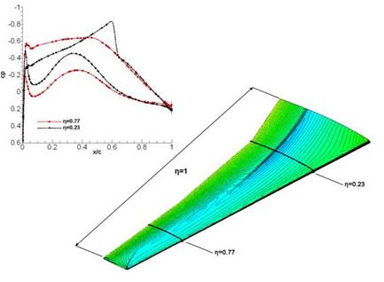
Fig. 11 Cp distribution of the SFB-401 wing. Cut at n=0.77 and 0.23

searches for the required TAU output files and reads in the results defined by the user before. Finally, the results of the ANOVA analysis are stored in a solution file, which can be easily read by Excel or other vizualisation tools. Validation of the pro­gram showed perfect agreement with the manual analysis and the required time is massively reduced as the hole setup for the TAU simulations is automatized. Still some knowledge about the Taguchi-Method is required. Therefore, a detailed users guide is added to the scripts including a detailed description of the Taguchi-Method and several examples.

Simulation Setup

To investigate the influence of different numerical parameters, steady and unsteady RANS simulations are performed. The TAU code developed by the DLR is used for all simulations. Test object is the RAE 2822 airfoil. The inflow conditions are chosen according to the known Case 9 [1].

Maoo = 0.73, T = 288.15K, Re = 6.5e+6, a = 2.80°

The following section gives a summary of the performed investigations and their results. As mentioned above the Taguchi method allows to evaluate also the influ­ence of the interactions between the parameters. Therefore, the different parameters are partitioned into several groups. Each group contained physically or numerically related parameters.

For the steady simulations (Run 1 till 5) the influences of each particular para­meter on the results for the lift coefficient Q, total drag coefficient Cd, pressure drag coefficient Cdp and viscous drag coefficient Cdv are investigated.

In case of the unsteady simulation the influence on the averaged lift and drag coefficients Cimean and Cdmean, their amplitudes ClA and CdA as well as their RMS values Clrms and Clrms is shown. Additionally, the influence on the buffet frequency is described.

All simulations are performed with the TAU-version 2008.1.1 and the meshes are all generated with GridGEN 15.11. The mesh generation is script based and all meshes are structured (C-mesh). For the mesh variation (Run 1 and 3) several differ­ent meshes are generated, each with another resolution, y+ value and grid resolution at leading and trailing edge. The mesh resolution is based on the number of points along the airfoil surface (upper and lower side).

No. of grid points:

19580 with 128 grid points on the airfoil surface,

79476 with 256 grid points on the airfoil surface,

320228 with 512 grid points on the airfoil surface,

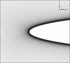
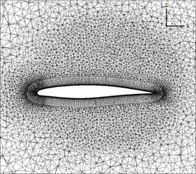
Figure 4 shows the leading edge region of the finest mesh with 512 points along the

airfoil surface. The TAU settings are chosen as follows:

k2-dissipation factor: 0.5

k4-dissipation factor: 64

CFL number: 1.5

Turbulence Model: Menter-SST

Simulation Setup

Fig. 4 Leading edge region of the finest mesh

4 Results

Run 1: Mesh resolution, Boundary layer resolution

Taguchi Matrix: L27

No. of levels: 3 for each parameter

Parameters: y+, Number of grid points on the airfoil surface,

mesh resolution leading edge, mesh resolution trailing edge

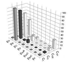
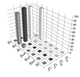
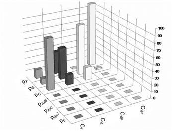
In the first case the influences of different grid parameters, including the y+ value, number of grid points on the airfoil surface, which determines the overall mesh resolution, as well as the local grid resolution at leading (LE) and trailing edge (TE) are evaluated. The last two mentioned properties are defined by the distance of the points on the airfoil surface. The mesh resolution at leading and trailing edge is set to coarse, medium and fine. The total value for each level depends on the total number of grid points on the surface. Defining the resolution at leading and trailing edge this way, guarantees meshes which are similar to each other. Table 1 gives an overview of the resulting total values, given in per mille of the chord length. The y+ value determines the height of the first cell row at the airfoil surface. The values for the three levels are 0.5, 1 and 2. Figure 5 shows the influences of the varied parameters on the coefficients for drag and lift given in percent. The influences of the interactions are shown as well. pAxC for examples denotes the influence of the interaction between parameters A and C. The error occurred during the ANOVA – analysis is given by pF. This value does not represent the influence of the error on the CFD result. It is just an indication for the certainty of the evaluated parameter influences. In this study only interactions with the y+ parameter are investigated. The reason is that four parameters are examined at once, and that there is no suitable Taguchi Matrix which includes four parameters and all their interactions. In Figure 5 it is shown that the influence of the number of grid points on the airfoils surface prevails in comparison to the other parameters. Especially for the results of lift, total drag and pressure drag. In case of the viscous drag also the y+ value shows some significant impact. This is due to the fact that this parameter effects the resolution of the boundary layer. The mesh resolution at trailing and leading edge shows only a small contribution. No interaction between the y+ value and the other parameters is detected.

Table 1 Total value of the grid point distance at leading and trailing edge for different mesh resolutions, given in per mille

Level

512

256

128

1-rough

1

2

4

2-middle

0.5

1

2

3-fine

0.25

0.5

1

Simulation Setup

Fig. 5 Results of run 1. A = y+, B = number of grid points on airfoil’s surface, C = mesh resolution TE, D = mesh resolution LE

Run 2: Inflow conditions

Taguchi Matrix: L27

No. of levels: 3 for each parameter

Parameters: Reynolds number, Mach number, angle of attack

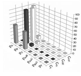
For the investigation on the inflow conditions the Reynolds number is varied by +/- 3 • 105, the Mach number by +/- 0.001 and the angle of attack by +/-0.01°. In this study the fine mesh with 512 grid points on the surface of the airfoil is chosen. The ANOVA analysis yields a large impact of the Reynolds number and the angle of attack on the lift coefficient Cl as it can be seen in Figure 6. This result is compre­hensible especially for the angle of attack. But it is also known that the lift increases with a rising Reynolds number. In transonic region the Mach number has a large influence on the total drag values because the pressure drag which is also mainly influenced by the Mach number has a large share in the total drag. The viscous drag, however, is only influenced by the Reynolds number. But it has only a low impact on the total drag.

Simulation Setup

Fig. 6 Results of run 2. A = Reynolds number, B = Mach number, C = angle of attack

Run 3: Turbulence modeling (a)

Taguchi Matrix: L27

No. of levels: 3 for each parameter

Parameters: Mesh resolution, CFL-number, numerical diffusion

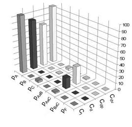
In this case the mesh resolution at leading and trailing edge is set to the medium value. The levels of the CFL number are set to 1.5, 3.25 and 5. The numerical dif­fusion terms are changed simultaneously. Their levels are (1/32; 1.00), (1/64; 0.50) and (1/128; 0.25) for k2 and k4 respectively. This study is done for several turbu­lence models like Menter-SST, Spalart Allmaras with Edwards correction (SAE), Linear Algebraic Stress Model (LEA) and for the Reynolds Stress Model (RSM). The results are very similar for all turbulence models. Therefore, only the result for the SAE model is exemplified in Figure 7. The analysis shows that the mesh res­olution has a main impact on all results again. The CFL number has no influence. This behaviour agrees well with the theory as long as all simulations are converged like in the present case. The influence of the numerical diffusion is also very small, but the interaction between the mesh resolution and the numerical diffusion shows a larger influence on the results. This is reasonable as the mesh has also a damping effect on the solution if it is too coarse. Since in this study only three parameters are investigated, the evaluation of all interaction effects is possible by using a L27 Matrix.

Simulation Setup

Fig. 7 Results of run 3. A = number of points on airfoil’s surface, B = CFL-number, C = Diffusion terms

Run 4: Turbulence modeling (b)

Taguchi Matrix: L27

No. of levels: 3 for each parameter

Parameters: Turbulence model, CFL-number, numerical diffusion

This is based on the results of run 3, which was performed for several turbulence models (Menter-SST, SAE, LEA). By rearranging the performed simulations, it is possible to replace the mesh resolution parameter by the turbulence model. A new ANOVA analysis shows that in this case the influence of the turbulence model out­balances all other parameters. This is not surprising because it is known that the turbulence model has a large impact on the CFD result, and the other parameters are not varied to such an extent to compete with the turbulence model.

Run 5: Geometry

Taguchi Matrix: L27

No. of levels: 3 for each parameter

Parameters: Trailing edge thickness, number of geometry-defining points,

bump height

The three levels of the trailing edge thickness are 0%, 0.5% and 1% of the chord length. The number of points defining the contour of the airfoil are set to 100, 200 and 400. Finally a sinus function is superposed with the leading edge contour to

Simulation Setup

Fig. 8 Results of run 5. A = number of geometry-defining points, B = Trailing edge thickness, C = Bump height.

simulate bump-shaped disturbances in the leading edge region. These bumps rep­resent the uncertainty in fabrication process. The amplitude levels of these bumps are set to 1 • 10~4, 2 • 10~4 and 3 • 10~4 times the chord length. For the simulation the mesh with 256 points on the airfoil’s surface is chosen. The trailing edge is dis­cretized with 56 cells and 110 cells for a trailing edge height of 0.5% and 1 % chord. The results show that the number of points has no influence. This is due to the fact that even 100 points are still sufficient to describe the airfoil’s contour nicely. The coefficients for lift, total drag and pressure drag are mainly affected by the trail­ing edge thickness while the viscous drag is influenced by the bump height. The bump height has an impact on the pressure distribution along the airfoil’s surface. The acceleration and deceleration along the wavy surface changes the load on the boundary layer which affects the viscous drag.

Run 6: Unsteady simulation

Taguchi Matrix: L27

No. of levels: 3 for each parameter

Parameters: CFL-number, Number of inner iterations, At

To get unsteady flow characteristics, the angle of attack is increased to 5°. For this angle of incidence buffet effects occur, i. e. that the shock on the upper surface starts to move with a distinct frequency. Therefore also the force coefficients fluctuate. In case of an unsteady simulation not only the mean force coefficients but also their

Simulation Setup

Fig. 9 Results of run 6. A = unsteady physical time step size; B = Number of inner iteration; C = CFL-number.

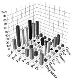
amplitudes, rms-values and frequencies can be analyzed. The CFL number is set to 3.4, 1.7 and 0.8 for the coarse multigrid and to 10, 5 and 2.5 for the fine multigrid. The ratio tchar to At is defined to 20, 40 and 80. Where tchar = UJc is the time the air needs to flow over the airfoil. The levels for the number of inner iterations are 50, 100 and 200. Looking at the results plotted in Figure 9 it must be said first that the CFL number has a larger impact on several results. As mentioned before this should not be the case if all simulations are converged. But in this study the inner iterations of some unsteady simulations are not converged. This explains the recognized influence of the CFL number. Furthermore, the unsteady physical time step size At/tchar has an influence on the mean values of the force coefficients and the frequency but not on the unsteady parts of the force coefficients, the rms-value and the amplitude. The unsteady physical time step size has also an indirect effect on all parameters through the interaction with the number of iterations. This interaction often has the strongest influence of all parameters. All other interaction effects can be neglected. The number of inner iterations has a direct influence on the frequency and the mean values.

Run 7: Robustness test

Taguchi Matrix: L27

No. of levels: 3 for each parameter

Parameters: Reynolds number, Mach number, angle of attack

The study for the inflow conditions is repeated, but the variation of the parameters is increased to three times the value as in run 2. The Mach number is now varied by +/-0.003, the angle of attack by +/-0.03° and the Reynolds number is varied by +/- 9 • 105. This study provides almost exactly the same results as run 2. This confirms the robustness of the Taguchi Method that shows that the obtained results are also valid for larger (or smaller) parameter variations.

Run 8: 3D Simulation

Taguchi Matrix: L27

No. of levels: 3 for each parameter

Parameters: Reynolds number, Mach number, angle of attack

Finally the Taguchi Method is used for the analysis of 3D simulations of the generic SFB-401 wing. Geometry and mesh are provided by the DLR. The mesh has 9.5 million points. The boundary layer is resolved with 80 layers in wall normal direc­tion. The boundary conditions are chosen to Ma = 0.8, Re = 23.5 • 106 and angle of attack of 1°. For the 3D simulation a Taguchi analysis of these boundary conditions is performed as it is already done for the RAE 2822 2D-airfoil shown before (Run 2). The variation of the Mach number is 0.001 and the angle of attack is varied by 0.01°. These variations are the same like in the investigation of the 2D-airfoil since the total values of these parameters are similar for the 3D and the 2D case. The Reynolds number is varied stronger than before as the Reynolds number of the 3D SFB-401 case is much higher than for the 2D test case. Therefore, it is varied by +/- 1 • 106 instead of +/-3 • 105. For the simulations the SAO turbulence model is used. The dissipation factors are set to 0.5 and 64 for k2 and k4 respectively. Figure 10 shows a cut through the mesh at n=0.77.

The cp distribution is shown in Figure 11. Inboard a shock appears due to super­sonic flow at x/c=0.6 for n=0.23. Further outboard at n=0.77 no shock is observed. These results are extracted from the simulation with Ma=0.799, Re=22.5 • 106 and angle of attack a=1.01°. The ANOVA analysis yielded results comparable to the 2D case but shows up also some differences (see Figure 12). The viscous drag is again mainly affected by the Reynolds number. Mach number and angle of attack have no influence. Looking on the pressure drag it can be recognized that the Mach number has the largest influence followed by the angle of attack which has some small contribution. The influence of the angle of attack is increased compared to the 2D airfoil as it has some impact on the induced drag which is a pressure drag as well and occurs only for lift producing 3D geometries. The results for the total drag show some differences to the 2D case. The impact of the Reynolds number is much higher for the 3D case. This can be explained by the larger contribution of the viscous drag to the total drag compared to the 2D case. For the 3D case the viscous drag is of the same size as the pressure drag while for the 2D case the pressure drag was twice the viscous drag. Therefore, the Reynolds number has a larger impact on the total drag for the 3D case. However, the influence of the Reynolds number on the

Simulation Setup

Fig. 10 Mesh of the SFB-401 wing. Cut at n=0.77

lift coefficient is smaller than in case of the 2D airfoil. This can be explained by the larger Reynolds number which is four times higher than for the 2D case. Therefore, the influence of the viscous forces on the lift will be smaller than for the 2D case. The higher contribution of the viscous drag to the total drag, mentioned before, is rather explained by a different geometry than by a different Reynolds number.

Error Determination

For each analysis the error can be calculated. During the investigations carried out at the IAG it was recognized that this error is very large if one or more simulations did not converge. This is obvious since the deviation caused by the non-convergence is usually larger than the deviation caused by the small parameter variations of the Taguchi analysis. Thus the convergence of every simulation is crucial and absolutely necessary for a reliable quantification of the parameter influences and interactions. The error that occurred can be evaluated similar to the influences in the ANOVA analysis.

No. of column

1

2

3

4

5

6

7

1

3

2

5

4

7

6

2

1

6

7

4

5

3

7

6

5

4

4

1

2

3

5

3

2

6

1

7

Fig. 3 Lg-Interaction-Matrix

The degree of freedom of the error term is calculated as follows,

Error Determination

i=1 j=1

Подпись: (13)

If the degree of freedom is non-zero, the error variance can be determined.

The degree of freedom becomes zero if all columns of the Taguchi matrix are oc­cupied with parameters. In this case an error determination as shown above is not possible. Instead the so-called pooling-method must be used. This method takes the parameters with the smallest influences to determine an error term. Following equation describes this method exemplarily for two parameters C and D.

Error Determination

Error Determination
Подпись: (12)

(15)

In [2] it is mentioned that at least half of the degrees of freedom ftotal should be used for this method to determine the error of the investigation. In the present investiga­tion all runs except run 1 are performed with Taguchi matrices which are not fully packed with parameters. Therefore usually the first error determination method is used.

Parameter Interaction

The influence of possible interactions between two parameters can be captured by the Taguchi Method as well. For each interaction one (for parameters with 2 levels) or two (for parameters with more than 2 levels) columns must be reserved in the orthogonal array. This increases the number of required columns and also the num­ber of simulations. Thus the advantage of requiring less simulations than a standard parameter variation is reduced. But on the other hand, the influence of interactions between the investigated parameters can be evaluated. This won’t be possible if a normal parameter simulation is used. For several pre-deflned Taguchi matrices so – called interaction-matrices are published. They describe which columns are reserved for which parameter interaction. The interaction-matrix for the Lg Matrix is shown in Figure 3. For example column 3 must be reserved to examine the interaction between the parameters number 1 and 2. The parameters originally stored in these columns would move to column 4 if no other interactions are investigated.

ANOVA-Analysis

With the ANOVA analysis (Analysis of Variances) the influence of each parameter and interaction on the result of the simulation is obtained. In this section a short summary of this statistical method is given. Thereby the variable y is the result of

Orthogonal

Array

Number of lines

Max. No. of parameters

Max. Number of columns for given Number of levels

2

3

4

5

L4

4

3

3

4

8

7

7

*"9

9

4

4

l12

12

11

11

*-16

16

15

15

*- 16

16

5

5

*"18

18

8

1

7

*“25

25

6

6

*"27

27

13

13

*"32

32

31

31

*" 32

32

10

1

9

*"36

36

23

11

12

*"36

36

16

3

13

*-50

50

12

1

11

к»

54

26

1

25

*"64

64

63

63

*" 64

64

21

21

*"81

81

40

40

Fig. 2 Overview about pre-defined Taguchi matrices

the CFD simulation, n is the number of simulations and f is the degree of freedom. First of all the mean square error is determined by

(V V’)2

SQin = -^-h— = CF. (1)

n

The degree of freedom of the mean square values is

fsQm = n – (n – 1) (2)

In the next step the total error square sum is determined.

SQtotal = (ZV»)2 – CF. (3)

ANOVA-Analysis
It has the degree of freedom

exemplarily shown for a parameter A with 3 levels. The results of the simulations with the same level for parameter A are summed, squared and divided by the number

of simulations with the same level of parameter A. Then the sum of the mean square values CF is subtracted. The degree of freedom is

fSQA = nLevels – fsQm, (6)

where nLevels are the number of levels of parameter A. The squared variances of the interactions are calculated by

SQm-b = і1У{АхВ)і) – CF – SQa – SQb, (7)

n(AxB)i

shown exemplarily for parameter A and B. The results of the simulations where the level combination of parameter A and B is the same are summed, squared and divided by the number of results with the same level combination. Then the sum of the mean square values and the mean square errors of parameter A and B are subtracted.

In the next step the estimation variances of each parameter are estimated by

again shown for parameter A. Then the evaluation of the critical Fi can be performed.

This value shown here for the parameter A is compared to the so called Fisher values. The Fisher value is a reference value used for the determination of the dif­ferences of variances with a certain probability of confidence. Reference values are given in so called Fisher tables depending on the probability of confidence. If the calculated Fisher value is larger than the value given by the Fisher table, the null hypothesis will be rejected. It is assumed that the differences from the total mean value are not random (null hypothesis). Therefore the alternative hypothesis is valid. If the null hypothesis is rejected, it can be assumed that an influence of the tested parameter is existent. For the percental influence of each parameter the adjusted error square sum must be determined first.

SQA = SQa – fAVF (10)

Dividing this value by the squared variances and multiplying it with 100. the per­centage influence of the parameter (here shown for parameter A) on the results of the simulation is obtained.

Orthogonal Arrays

The simulation procedure is described by orthogonal arrays called Taguchi matrices. Such an array is based on the number of variables and their interactions (columns) plus the number of levels which yield the number of lines. Usually a pre-defined matrix is chosen, but it is also possible to design a new matrix or to adapt an existing matrix. In Figure 1a L9 matrix is shown, which is suitable for the evaluation of the influence of 4 parameters with 3 levels each. The first column shows the number of the simulation. The following 4 columns (A-D) describe the settings for the 4 parameters. The results of the 9 simulations are recorded in the last column. The matrix describes the setting for each parameter. For example in simulation number 4 the parameter A is set to level 2, parameter B to level 1, parameter C to level 2 and parameter D is set to level 3. Several pre-defined matrices exist, shown in Figure 2 for different numbers of parameters and levels.

A modification of these matrices is possible. For example, the number of levels of a chosen parameter can be increased or reduced. But it has to be kept in mind that the sum of the degrees of freedom for all columns is not higher than the degree of freedom of the whole matrix. The degree of freedom of one column is equal to the number of levels minus 1 while the degree of freedom of the matrix is the number of simulations minus 1.

After all simulations have been done, the influence of each parameter is determ­ined by an statistical ANOVA-Analysis (Analysis of Variances).