Category THEORETICAL AERODYNAMICS

The third vortex theorem of Helmholtz’s states that:

“the circulation of a vortex tube remains constant in time."

Using Helmholtz’s second theorem and Kelvin’s circulation theorem, the above statement can be inter­preted as “a closed line generating the vortex tube is a material line whose circulation remains constant.” Helmholtz’s second and third theorems hold only for inviscid and barotropic fluids.

5.9.2 Helmholtz’s Fourth Vortex Theorem

The fourth theorem states that:

“the strength of a vortex remains constant in time."

This is similar to the fact that the mass flow rate through a streamtube is invariant as the tube moves in the flow field. In other words, the circulation distribution gets adjusted with the area of the vortex tube. That is, the circulation per unit area (that is, vorticity) increases with decrease in the cross-sectional area of the vortex tube and vice versa.

The second vortex theorem of Helmholtz’s states that:

“a vortex tube is always made up of the same fluid particles."

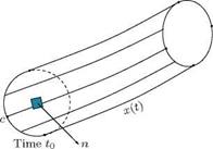
In other words, a vortex tube is essentially a material tube. This characteristic of a vortex tube can be represented as a direct consequence of Kelvin’s circulation theorem. Let us consider a vortex tube and an arbitrary closed curve c on its surface at time t0, as shown in Figure 5.30. By Stokes integral theorem, the circulation of the closed curve c is zero (that is, Dr/Dt = 0). The circulation of the curve, which is made up of the same material particles, still has the same (zero) value of circulation at a latter instant of time t.

y inverting the above reasoning, it follows from Stokes integral theorem that these material particles must be on the outer surface of the vortex tube.

If we examine smoke-rings, it can be seen that the vortex tubes are material tubes. The smoke will remain in the vortex ring and will be transported with it, so that it is the smoke itself which carries the vorticity. This statement holds under the restrictions of barotropy (that is, p = p(p), the density is a function of pressure only) and zero viscosity. The slow disintegration seen in smoke-rings is due to friction and diffusion. A vortex ring which consists of an infinitesimally thin vortex filament induces an infinitely large velocity on itself (similar to the horseshoe vortex), so that the ring would move forward with infinitely large velocity. The induced velocity at the center of the ring remains finite (as in horseshoe vortex). From Biot-Savart law, the induced velocity becomes:

_ Г Г2 h2dф _ Г 4 ж 0 h3 2 h

This velocity becomes infinitely large (that is, unrealistic) when the cross-section of the vortex ring is assumed to be infinitesimally small. For finite cross-section, the velocity induced by the ring on itself, that is, the velocity with which the ring moves forward remains finite. But in reality the actual cross-section of the ring is not known, and probably depends on how the ring was formed.

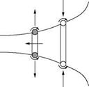
In practice we notice that the ring moves forward with a velocity which is slower than the induced velocity in the center. Also, it is well known that two rings moving in the same direction continu­ally overtake each other whereby one slips through the other in front. This phenomenon, illustrated in Figure 5.31, is explained by mutually induced velocities on the rings and formula given above for the velocity at the center of the ring.

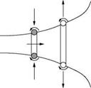
In a similar manner it can be explained why a vortex ring towards a wall becomes larger in diameter and at the same time its velocity gets reduced. Also, the diameter decreases and the velocity increases when a vortex ring moves away from a wall, as illustrated in Figure 5.32.

To work out the motion of vortex rings the cross-section of vortex must be known. Further, for in­finitesimally thin rings the calculation fails because vortex rings, such as curved vortex filaments, induce large velocities on themselves. However, for straight vortex filaments, that is, for vortex filaments in two-dimensional flows, a simple description of the “vortex dynamics” for infinitesimally thin filaments is possible, since for such a case the self-induced translational velocity vanishes. We know that vortex filaments are material lines, therefore it is sufficient to calculate the paths of the fluid particles which carry the rotation in xy-plane perpendicular to the filaments, using:

Figure 5.32 Kinematics of a vortex ring near a wall.

that is, to determine the paths of the vortex centers. The induced velocity which a straight vortex filament at position xi induces at position x is known from Equation (5.49), that is:

v = ——- (cos a + cos 0) .

4nh

As we have seen, the induced velocity is perpendicular to the vector hi = ri = (x – xi), and therefore

hi

has the direction ez x ——, so that the vectorial form of Equation (5.41) reads as:

|hi|

Г

UR = ez x

2 n

For x ^ xi the velocity tends to infinity, but because of symmetry the vortex cannot be moved by its own velocity field, that is, the induced translational velocity is zero. The induced velocity of n vortices with the circulation Г (i = 1, 2, … n) is:

ur = ri<

2 n

If there are no internal boundaries, or if the boundary conditions are satisfied by reflection, as in Figure 5.32, the last equation describes the entire velocity field, and using dx/dt = u(x, t) or dxi/dt = ui(xi, t), the “equation of motion” of the kth vortex becomes:

For i = k, the induced translational velocity becomes zero, owing to symmetry, and hence excluded from the summation. Equation (5.58) gives the 2n relations for the path coordinates.

The dynamics of vortex motion have invariants which are analogous to the invariants of a point mass system on which no external forces act. The conservation of strengths of the vortices by Helmholtz’s theorem (^ Гк = constant) corresponds to mass conservation of total mass of the point mass system. When the Equation (5.58) is multiplied by Гк, summed over к and expanded, we get:

In the above equation, the terms on the right-hand side cancel out in pairs, and the equation reduces to:

On integration this results in:

k

The integration constants are written as xg, which is like a center of gravity coordinate (this is done here for dimensional homogeneity). Equation (5.59) states that:

“the center of gravity of the strengths of the vortices is conserved."

For a point mass system, by conservation of momentum, we have the corresponding law, namely: “the velocity of the center of gravity is a conserved quantity in the absence of external forces."

For ^ Гк — 0, the center of gravity lies at infinity, so that, for example, two vortices with Г1 — – Г2 must take a turn about a center of gravity point Pg which is at a finite distance, as shown in Figure 5.33.

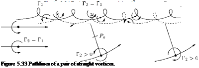The paths of the vortex pairs are determined by numerical integration of Equation (5.58). The paths will look like those shown in Figure 5.34.

A vortex is termed semi-infinite vortex when one of its ends stretches to infinity. In our case let the end B in Figure 5.24 stretches to infinity. Therefore, в = 0 and cos в = 1, thus, from Equation (5.49), we have the velocity induced by a semi-infinite vortex at a point P as:

Г

v =—— (cos a + 1). (5.50)

4nh

5.9.1 Infinite Vortex

An infinite vortex is that with both ends stretching to infinity. For this case we have a = в = 0. Thus, the induced velocity due to an infinite vortex becomes:

Г

2nh

For a specific case of point P just opposite to one of the ends of the vortex, say A, we have a = n/2 and cos a = 0. Thus, the induced velocity at P becomes:

Г

4nh

This amounts to precisely half of the value for the infinitely long vortex filament [Equation (5.51)], as we would expect because of symmetry.

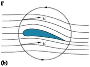
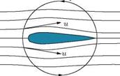
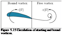
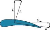
While discussing Figure 5.15, we saw that the circulation about an aerofoil in two-dimensional flow can be represented by a bound vortex. We can assume these bound vortices to be straight and infinitely long vortex filaments (potential vortices). As far as the lift is concerned we can think of the whole aerofoil as being replaced by the straight vortex filament. The velocity field close to the aerofoil is of course different from the field about a vortex filament in cross flow, but both fields become more similar when the distance of the vortex from the aerofoil becomes large.

In the same manner, a starting vortex can be assumed to be a straight vortex filament which is attached to the bound vortex at plus and minus infinity. The circulation of the vortex determines the lift, and the lift formula which gives the relation between circulation, Г, and lift per unit width, l, in inviscid potential flow is the Kutta-Joukowski theorem,6 namely:

l =-рГиж, (5.53)

where l is the lift per unit span of the wing, Г is circulation around the wing, иж is the freestream velocity and p is the density of the flow.

It is important to note that the lift force on a wing section in inviscid (potential) flow is perpendicular to the direction of the undisturbed stream and thus an aerofoil experiences only lift and no drag. This result is of course contrary to the actual situation where the wing experiences drag also. This is because here in the present approach the viscosity of air is ignored whereas in reality air is a viscous fluid. The Kutta-Joukowski theorem in the form of Equation (5.53) with constant Г holds only for wing sections in a two-dimensional plane flow. In reality all wings are of finite span and hence the flow essentially becomes three-dimensional. But as long as the span is much larger than the chord of the wing section, the lift can be estimated assuming constant circulation Г along the span. Thus, the lift of the whole wing span 2b is given by:

But in reality there is flow communication from the bottom to the top at the wing tips, owing to higher pressure on the lower surface of the wing than the upper surface. Therefore, by Euler equation, the fluid flows from lower to upper side of the wing under the influence of the pressure gradient, in order to even 6The Kutta-Joukowski theorem is a fundamental theorem of aerodynamics. It is named after the German Martin Wilhelm Kutta and the Russian Nikolai Zhukovsky (or Joukowski) who first developed its key ideas in the early 20th century. The theorem relates the lift generated by a right cylinder to the speed of the cylinder through the fluid, the density of the fluid, and the circulation. The circulation is defined as the line integral, around a closed loop enclosing the cylinder or aerofoil, of the component of the velocity of the fluid tangent to the loop. The magnitude and direction of the fluid velocity change along the path.

The flow of air in response to the presence of the aerofoil can be treated as the superposition of a translational flow and a rotational flow. It is, however, incorrect to think that there is a vortex like a tornado encircling the cylinder or the wing of an airplane in flight. It is the integral’s path that encircles the cylinder, not a vortex of air. (In descriptions of the Kutta-Joukowski theorem the aerofoil is usually considered to be a circular cylinder or some other Joukowski aerofoil.)

The theorem refers to two-dimensional flow around a cylinder (or a cylinder of infinite span) and determines the lift generated by one unit of span. When the circulation Г ж is known, the lift L per unit span (or l) of the cylinder can be calculated using the following equation:

l = рто^тоГто?

where рж and Vж are the density and velocity far upstream of the cylinder, and Г ж is the circulation defined as the line integral,

Г ж = V cos 9ds

around a path c (in the complex plane) far from and enclosing the cylinder or airfoil. This path must be in a region of potential flow and not in the boundary layer of the cylinder. The V cos 9 is the component of the local fluid velocity in the direction of and tangent to the curve c, and ds is an infinitesimal length on the curve c. The above equation for lift l is a form of the Kutta-Joukowski theorem.

The Kutta-Joukowski theorem states that, “the force per unit length acting on a right cylinder of any cross section whatsoever is equal to PжVжГж, and is perpendicular to the direction of Vж”
out the pressure difference. In this way the magnitude of the circulation on the wing tips tends to become zero. Therefore, the circulation over the wing span varies and the lift is given by:

■+ b

Г(х) dx,

b

where the origin is at the middle of the wing, x is measured along the span, and b is the semi-span of the wing.

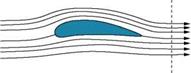
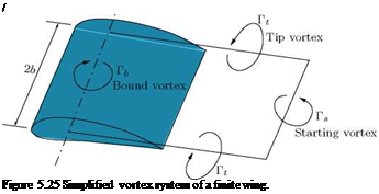
According to Helmholtz’s first vortex theorem, being purely kinematic, the above relations for lift are also valid for the bound vortex. Thus, isolated pieces of a vortex filament cannot exist. Also, it cannot continue to be straight along into infinity, where the wing has not cut through the fluid and thus no discontinuity surface has been generated as is necessary for the formation of circulation. Therefore, free vortices, Г, which are carried away by the flow must be attached at the wing tips. Together with the bound vortex, Гь, and the starting vortex, Ts, they (the tip vortices) form a closed vortex ring frame in the fluid region cut by the wing, as shown in Figure 5.25.

If a long time has passed since start-up, the starting vortex is at infinity (far downstream of the wing), and the bound vortex and the tip vortices together form a horseshoe vortex.

Even though the horseshoe vortex system represents only a very rough model of a finite wing, it can provide a qualitative explanation for how a wing experiences a drag in inviscid flow, as already mentioned. The velocity w induced at the middle of the wing by the two tip vortices accounts for double the velocity induced by a semi-infinite vortex filament at distance b. Therefore, by Equation (5.50), we have:

This velocity is directed downwards and hence termed induced downwash. Thus, the middle of the wing experiences not only the freestream velocity Ux, but also a velocity u, which arises from the superposition of Ux and downwash velocity w, as shown in Figure 5.26.

In inviscid flow, the force vector is perpendicular to the actual approach direction of the flow stream, and therefore has a component parallel to the undisturbed flow, as shown in Figure 5.26, which manifests itself as the induced drag Di, given by:

w

Di — A.

U

It is important to note that Equation (5.57) holds if the induced downwash from both vortices is constant over the span of the wing. However, the downwash does change since at a distance x from the wing center, one vortex induces a downwash of:

Г

4 n (b + x) ’

whereas the other vortex induces:

Г

4 n (b — x)

Both the downwash are in the same direction, therefore adding them we get the effective downwash as:

ГГ w — +

4 n (b + x) 4 n (b — x)

_ Г 2b

4 n b2 — x2

_ Г b

2 n b2 — x2

From this it can be concluded that the downwash is the smallest at the center of the wing (that is, Equation (5.57) underestimates the induced drag) and tends to infinity at the wing tips. The unrealistic value there (at wing tips) does not appear if the circulation distribution decreases towards the wing tips, as in deed it has to. For a semi-elliptical circulation distribution over the span of the wing, the downwash distribution becomes constant and Equation (5.57) is applicable. Helmholtz first vortex theorem stipulates that for an infinitesimal change in the circulation in the x-direction of:

dT

dr — dx dx

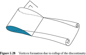
and a free vortex of the same infinitesimal strength must leave the trailing edge. This process leads to an improved vortex system, as shown in Figure 5.27.

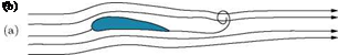
The free vortices form a discontinuity surface in the velocity components parallel to the trailing edge, which rolls them into the kind of vortices, as shown in Figure 5.28.

These vortices must be continuously renewed as the wing moves forward. This calls for continuous replenishment of kinetic energy in the vortex. The power needed to do this is the work done per unit time by the induced drag.

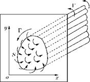
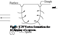
The manifestation of Helmholtz’s first theorem can be encountered in daily life. Recall the dimples formed at the free surface of coffee in a cup when a spoon is suddenly dipped into it. The formation process of dimples looks like that shown schematically in Figure 5.29.

As the fluid flows together from the front and back, a surface of discontinuity forms along the rim of the spoon. The discontinuity surface rolls itself into a bow-shaped vortex whose endpoints form the dimples on the free surface, as shown in Figure 5.29.

The flow outside the vortex filament is a potential flow. Thus, by incompressible Bernoulli equation, we have:

This is valid both along a streamline and between any two points in the flow field.[5] Also, at the free surface the pressure is equal to the ambient pressure pa. Further, at some distance away from the vortex the velocity is zero and there is no dimple at the free surface, and hence z = 0. Thus, the Bernoulli constant is equal to pa and we have:

2

2 pu + pgz = 0.

Near the end points of the vortex the velocity increases by the formula given by Equation (5.52), and therefore z must be negative, that is, a depression of the free surface. In reality, the cross-sectional surface of the vortex filament is not infinitesimally small, therefore we cannot take the limit h ^ 0 in Equation (5.52), for which the velocity becomes infinite. However, the induced velocity due to the vortex filament is so large that it causes a noticeable formation of dimples.

It should be noted that an infinitesimally thin filament cannot appear in actual flow because the velocity gradient of the potential vortex tends to infinity for h ^ 0, so that the viscous stresses cannot be ignored even for very small viscosity. Also, it is well known that the viscous stresses make no contribution to particle acceleration in incompressible potential flow, but they do deformation work and thus provide a contribution to the dissipation. The energy dissipated in heat stems from the kinetic energy of the vortex.

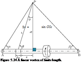
Examine the linear vortex of finite length AB, shown in Figure 5.24. Let P be an adjacent point located by the angular displacements a and в from A and B respectively. Also, the point P has coordinates r and O with respect to an elemental length Ss of AB. Further, h is the height of the perpendicular from P to AB, and the foot of the perpendicular is at a distance s from Ss.

The velocity induced at P by the element of length Ss, by Equation (5.47), is:

The induced velocity is in the direction normal to the plane ABP, shown in Figure 5.24.[4]

The velocity at P due to the length AB is the sum of induced velocities due to all elements, such as Ss. However, all the variables in Equation (5.48) must be expressed in terms of a single variable before integrating to get the effective velocity. A variable such as ф, shown in Figure 5.24 may be chosen for

this purpose. The limits of integration are:

Фа=-(2-a)toфв=+(2-p), since ф passes through zero while integrating from A to B. Here we have:

sin в = cos ф r2 = h2 sec2 ф

ds = d (h tan ф) = h sec2 фdф.

Thus, we have the induced velocity at P due to vortex AB, by Equation (5.48), as:

This is an important result of vortex dynamics. From this result we obtain the following specific results of velocity in the vicinity of the line vortex.

Biot-Savart law relates the intensity of magnitude of magnetic field close to an electric current carrying conductor to the magnitude of the current. It is mathematically identical to the concept of relating intensity of flow in the fluid close to a vorticity-carrying vortex tube to the strength of the vortex tube. It is a pure kinematic law, which was originally discovered through experiments in electrodynamics. The vortex filament corresponds there to a conducting wire, the vortex strength to the current, and the velocity field to the magnetic field. The aerodynamic terminology namely, “induced velocity” stems from the origin of this law.

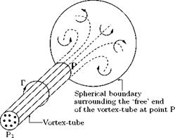
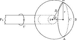
Now let us calculate the induced velocity at a point in the field of an elementary length Ss of a vortex of strength Г. Assume that a vortex tube of strength Г, consisting of an infinite number of vortex filaments, to terminate in some point P, as shown in Figure 5.21.

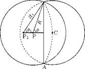
The total strength of the vortex tube will be spread over the surface of a spherical boundary of radius R. The vorticity in the spherical surface will thus have the total strength of Г. Because of symmetry the velocity of flow at the surface of the sphere will be tangential to the circular line of intersection of the sphere with a plane normal to the axis of the vortex tube. Such plane will be a circle ABC of radius r subtending a conical angle 26 at P, as shown in Figure 5.22.

If the velocity on the sphere at (R, 6) from P is v, then the circulation round the circuit ABC is Г’, where:

Г’ = 2nR sin 6 v.

The radius of the circuit is r = R sin в, therefore, we have:

Г’ = 2nr v.

But the circulation round the circuit is equal to the strength of the vorticity in the contained area. This is on the cap ABCD of the sphere. Since the distribution of the vorticity is constant over the surface, we have:

, Surface area of the cap 2nR2 (1 — cos в)

Г’ = —————————– — Г = ——— 2————– Г,

Surface area of the sphere 4nR2

that is:

(5.43)

From Equations (5.42) and (5.43), we obtain the induced velocity as:

Г

v =——- (1 — cos 9). (5.44)

4лг

Now, assume that the length of the vortex decreases until it becomes very short, as shown (PjP) in Figure 5.23. The circle ABC is influenced by the opposite end Pj also (that is, both the ends P and P’ of the vortex influence the circle). Now the vortex elements entering the sphere are congregating on Pj. Thus, the sign of the vorticity is reversed on the sphere of radius Rj. The velocity induced at Pj becomes:

Г

vj =——— (1 — cos 9j). (5.45)

4лг

The net velocity on the circuit ABC is the sum of Equations (5.44) and (5.45), therefore, we have:

Ц — cos 9) — Ц — cos 9j)

(cos 9i — cos 9).

As the point Pj approaches P,

(9 — S9) = cos 9 + sin 9 S9

and

(v — vj) ^ Sv.

Thus, at the limiting case of Pj approaching P, we have the net velocity as:

Г

Sv = —- sin 9S9. (5.46)

4лг

This is the velocity induced by an elementary length Ss of a vortex of strength Г which subtends an angle S9 at point P located by the ordinate (R, 9) from the element. Also, r = R sin 9 and RS9 = Ss sin 9, thus

It is evident from Equation (5.47) that to obtain the velocity induced by a vortex this equation has to be integrated. This treatment of integration varies with the length and shape of the finite vortex being studied. In our study here, for applying Biot-Savart law, the vortices of interest are all nearly linear. Therefore, there is no complexity due to vortex shape. The vortices will vary only in their overall length.

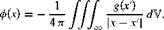
We see that Equation (5.24) is satisfied if uR is represented as the curl of a new, yet unknown, vector field a. Thus:

We can express Equation (5.30) as:

v x u = v (V • a) — Aa. (5.31)

Up to now the only condition on vector a is to satisfy Equation (5.28). But this condition does not uniquely determine this vector, because we can always add the gradient of some other function f to a without changing Equation (5.28), since v x v f = 0. If, in addition, we want the divergence of a to vanish (that is, v • a = 0), we obtain from Equation (5.31) the simpler equation:

V x u = — Aa. (5.32)

In this equation, let us consider v x u as a given vector function b(x), which is determined by the choice of the vector filament and its strength (that is, circulation). Thus, the Cartesian component form of the vector Equation (5.32) leads to three Poisson’s equations, namely:

Aa; = — b;; i = 1, 2, 3. (5.33)

For each of these component equations, we can apply the solution [Equation (5.27)] of Poisson’s equation. Now, vectorially combining the result, we can write the solution for a, from Equation (5.32), in short as:

Thus, calculation of the velocity field u(x) for a given distribution g(x) = div u and b(x) = curl u is reduced to the following integration processes, which may have to be done numerically:

Now, let us calculate the solenoidal term of the velocity uR, using Equation (5.35). This is the only term in incompressible flow without internal boundaries. Consider a field which is irrotational outside the vortex filament, shown in Figure 5.20.

The velocity field outside the filament is given by:

Stoke’s theorem relates the surface integral over an open surface to a line integral along the bounded curve. Let S be a simply connected surface, which is otherwise of arbitrary shape, whose boundary is c, and let u be any arbitrary vector. Also, we know that any arbitrary closed curve on an arbitrary shape can be shrunk to a single point. The Stoke’s integral theorem states that:

“The line integral J u ■ dx about the closed curve c is equal to the surface integral JJ (v x u) ■ nds over any surface of arbitrary shape which has c as its boundary."

That is, the surface integral of a vector field u is equal to the line integral of u along the bounding curve:

where dx is an elemental length on c, and n is unit vector normal to any elemental area on ds, as shown in Figure 5.17.

Stoke’s integral theorem allows a line integral to be changed to a surface integral. The direction of integration is positive counter-clockwise as seen from the side of the surface, as shown in Figure 5.17.

Helmholtz’s first vortex theorem states that:

“the circulation of a vortex tube is constant along the tube."

A vortex tube is a tube made up of vortex lines which are tangential lines to the vorticity vector field, namely curl u (or f). A vortex tube is shown in Figure 5.18. From the definition of vortex tube it is evident

curl u

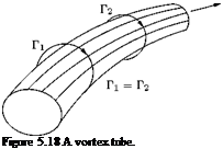that it is analogous to the streamtube, where the flow velocity is tangential to the streamlines constituting the streamtube. A vortex line is therefore related to the vorticity vector in the same way the streamline is related to the velocity vector. If Zx, Zy and Zz are the Cartesian components of the vorticity vector Z, along x-, y – and z-directions, respectively, then the orientation of a vortex line satisfies the equation:

along a streamline. In an irrotational vortex (free vortex), the only vortex line in the flow field is the axis of the vortex. In a forced vortex (solid-body rotation), all lines perpendicular to the plane of flow are vortex lines.

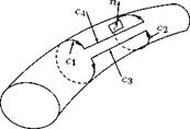
Now consider two closed curves c1 and c2 in a vortex tube, as shown in Figure 5.19.

According to Stoke’s theorem, the two line integrals over the closed curves in Figure 5.19 vanish, because the integrand on the right-hand side of Equation (5.13) is zero, since curl u is, by definition, perpendicular to n. The contribution to the integral from the infinitely close segments c3 and c4 of the curve cancel each other, leading to the equation:

u ■ dx + / u ■ dx = 0,

c1 J c2

since the distance between the segments c3 and c4 are infinitesimally small, we ignore that and treat c1 and c2 to be closed curves. By changing the direction of integration over c2, thus changing the sign of the second integral in Equation (5.14), we obtain Helmholtz’s first vortex theorem.
(5.15)
Derivation of this equation clearly demonstrates the kinematic nature of Helmholtz’s first vortex theorem. Another approach to the physical explanation of this theorem stems from the fact that the divergence of the vorticity vector vanishes. That is, the vorticity vector field curl u can be considered as analogous to an incompressible flow (for which the divergence of velocity is zero). In other words, the vortex tube becomes the streamtube of the new field. Now applying the continuity equation in its integral form (that is, JJs puiUi ds = 0) to a part of this streamtube, and at the same time replacing u by curl u, we get.
p (curl u) ■ nds = 0.
Since p is a constant, we can write this as.
(5.16)
(curlu) ■ nds = 0,
that is, for every closed surface s, the flux of the vorticity is zero. Applying Equation (5.16) to a part of the vortex tube whose closed surface consists of the surface of the tube and two arbitrarily oriented cross-sections A1 and A2, we obtain.
	(5.17)
since the integral over the tube surface vanishes. The integral.
(curlu) ■ nds
is called the vortex strength. It is identical to the circulation. From Equation (5.17) it is evident that. “the vortex strength of a vortex tube is constant." Noting the sense of integration of the line integral, Stoke’s theorem transforms Equation (5.17) into Helmholtz’s first theorem [Equation (5.15)]. From this representation it is obvious that, just like the streamtube, the vortex tube also cannot come to an end within the fluid, since the amount of fluid which flows through the tube (in unit time) cannot simply vanish at the end of the tube. The tube must either reach out to infinity (that is, should extend to infinity), or end at the boundaries of the fluid, or close around into itself and, in the case of a vortex tube, form a vortex ring. A very thin vortex tube is referred to as a vortex filament. The vortex filaments are of particular importance in aerodynamics. For a vortex filament the integrand of the surface integral in Stoke’s theorem

[Equation (5.13)]:

can be taken in front of the integral to obtain:

(curl u) • nAs = Г (5.19)

or

2a • n As = 2a As = constant, (5.20)

where a is the angular velocity. From this it is evident that the angular velocity increases with decreasing cross-section of the vortex filament.

It is a usual practice to idealize a vortex tube of infinitesimally small cross-section into a vortex filament. Under this idealization, the angular velocity of the vortex, given by Equation (5.20), becomes infinitely large. From the relation:

a As = constant,

we have a ^ ж, for As ^ 0.

The flow field outside the vortex filament is irrotational. Therefore, for a vortex of strength Г at a particular position, the spatial distribution of curl и is fixed. In addition, if div и is also given (for example, div и = 0 in an incompressible flow), then according to the fundamental theorem of vortex analysis, the velocity field и (which may extend to infinity) is uniquely determined provided the normal component of velocity vanishes asymptotically sufficiently fast at infinity and no internal boundaries exist.

The fundamental theorem of vector analysis is also essentially purely kinematic in nature. Therefore, it is valid for both viscous and inviscid flows, and not restricted to inviscid flows only. Let us split the velocity vector и into two parts, namely due to potential flow and rotational flow. Therefore:

U — Uir + Ur, (5.22)

where u! R is velocity of irrotational flow field and uR is velocity of rotational flow field. Thus, u! R is velocity of an irrotational flow field, that is:

curl u! R = v x uR = 0, (5.23)

The second is a solenoidal (coil like shape) flow field, thus:

divuR = v • uR = 0. (5.24)

Note that Equation (5.23) is the statement that “the vorticity of a potential flow is zero” and Equation (5.24) is the statement of continuity equation of incompressible flow.

The combined field is therefore neither irrotational nor solenoidal. The field u! R is a potential flow, and thus in terms of potential function ф, we have u! R = v ф. Let us assume that the divergence u to be a given function g(x). Thus:

div u — v • uir + v • ur — g(x),

div u = v • uir = g(x),

since v • uR = 0. Also, u! R = v ф. Therefore:

V2Ф = g (x)

(5.26)

This is an inhomogeneous Laplace equation, also called Poisson’s equation. The theory of this partial differential equation is the subject of potential theory which plays an important role in many branches of physics as in fluid mechanics. It is well known from the results of potential theory that the solution of Equation (5.26) is given by:

(5.27)

where x is the place where the potential ф is calculated, and x’ is the abbreviation for the integration variables xj, x’2 and x’3, and dV = (dx[dx’2dx’3) is a differential volume. The domain to implies that the integration is to be carried out over the entire space. Vortex Theorems Posted by admin in THEORETICAL AERODYNAMICS on March 18, 2016 Now let us have a closer look at the theorems governing vortex motion. Consider the circulation of a closed material line. By definition (Equation 5.3), we have the circulation as: The time rate of change of Г can be expressed as: (5.7) since ds/dt = V, where V is the velocity, s is length and t is time. The second integral in Equation (5.7) vanishes, since V ■ dV = d ^V ■ is the total differential of a single valued function, and the starting point of integration coincides with the end point. By Euler equation, we have: where FB is the body force. From Equation (5.7) and the Euler equation, we obtain the rate of change of the line integral over the velocity vector in the form: (5.8) In Equation (5.8), Dr/Dt vanishes if (FB ■ ds) and yр/р can be written as total differentials. When the body force FB has a potential (that is, when the body force is a conservative force field); implying that the work done by the weight in taking a body from a point P to another point Q is independent of the path taken from P to Q, and depends only on the potential, the first closed integral in Equation (5.8) becomes zero because: FB ■ ds =— y ф ■ ds =— d^. For a homogeneous density field or in barotropic flow, the density depends only on pressure, that is р = f (p). For such a flow, the second term on the right-hand side of Equation (5.8), can be expressed as: Therefore, for barotropic fluids, the second integral also vanishes in Equation (5.8). Equations (5.8) to (5.10) form the content of Thompson’s vortex theorem or Kelvin’s circulation theorem. This theorem states that: “in a Bow of inviscid and barotropic fluid, with conservative body forces, the circulation around a closed curve (material line) moving with the fluid remains constant with time, " if the motion is observed from a nonrotating frame. The vortex theorem can be interpreted as follows: “The position of a curve c in a flow field, at any instant of time, can be located by following the motion of all the fluid elements on the curve. " That is, Kelvin’s circulation theorem states that, the circulation around the curve c at the two locations is the same. In other words: where D/Dt(= d/dt + V • has been used to emphasize that the circulation is calculated around a material contour moving with the fluid. With Kelvin’s theorem as the starting point, we can explain the famous Helmholtz’s vortex theorem, which allows a vivid interpretation of vortex motions which are of fundamental importance in aerody­namics. Before venturing to explain Helmholtz’s vortex theorems, it would be beneficial if we consider the origin of the circulation around an aerofoil, in a two-dimensional potential flow, because Kelvin’s theorem seems to contradict the formulation of this circulation. It is well known that, the force on an aerofoil in a two-dimensional potential flow is proportional to the circulation. Also, the lift, namely the force perpendicular to the undisturbed incident flow direction, experienced by the aerofoil is directly proportional to the circulation, T, around the aerofoil. The lift per unit span of an aerofoil can be expressed as: where p and V, respectively, are the density and velocity of the freestream flow. Now let us examine the flow around a symmetrical and an unsymmetrical aerofoil in identical flow fields, as shown in Figure 5.12. As seen from Figure 5.12(a), the flow around the symmetrical aerofoil at zero angle of incidence is also symmetric. Therefore, there is no net force perpendicular to the incident (a) Figure 5.12 (a) Symmetrical and (b) unsymmetrical aerofoil in uniform flow. A A’   Figure 5.13 Velocity on either side of separation surface behind the aerofoil. flow direction. The contribution of the line integral of velocity about the upper-half of the aerofoil to the circulation has exactly the same magnitude as the contribution of the line integral of velocity about the lower-half, but with opposite sign. Therefore, the total circulation around the symmetric aerofoil is zero. The flow around the unsymmetrical aerofoil, as shown in Figure 5.12(b), is asymmetric. The contribu­tion of the line integral of velocity about upper-half of the aerofoil has an absolute value larger than that of the contribution about the lower-half. Therefore, the circulation around the unsymmetrical aerofoil is nonzero. By Bernoulli theorem it can be inferred that the velocity along a streamline which runs along the upper-side of the aerofoil is larger on the whole than the velocity on the lower-side. Therefore, the pressure on the upper side is less than the pressure on the lower side. Thus there is a net upward force acting on the aerofoil. For an unsymmetrical aerofoil the flow velocity over the upper and lower surfaces are different even when it is at zero angle of incidence to the freestream flow. Because of this the pressure on either side of the dividing streamline, shown in Figure 5.13, are different. Also, the velocities on either side of the separation surface are different, as shown in the figure. This implies that the pressure on either side of the separation surface are different. It is well known that the separation surface, which is also called slipstream, cannot be stable when the pressures on either side are different [4]. The slipstream will assume a shape in such a manner to have equal pressure on either side of it. Here the pressure at the lower side is higher than that at the upper side. Thus, the slipstream bends up, as shown in Figure 5.14(a). At the first instant of start-up, the flow around the trailing edge of the aerofoil is at very high velocities. Also, the flow becomes separated from the upper surface. Flow field around an aerofoil at different phases of start-up is shown in Figure 5.14. The separation at the upper surface is caused by the very large deceleration of the flow from the maximum thickness location to the separation point S, which is formed on the upper surface since the flow is still circulation-free flow [Figure 5.14(a)]. This flow separates from the upper surface even with very little viscosity (that is, g ^ 0) and forms the wake, which becomes the discontinuity surface in the limiting case of g = 0. The flow is irrotational everywhere except the wake region. Soon after start-up, the separation point is dipped to the trailing edge, as per Kutta hypothesis, and the slipstream rolls-up as shown in Figure 5.14(b). The vortex thus formed is pushed downstream and positioned at a location behind the aerofoil, as shown in Figure 5.14(c). This vortex is called starting vortex. The starting vortex is essentially a free vortex because it is formed by the kinematics of the flow and not by the viscous effect. By Kelvin’s circulation theorem, a closed curve which surrounds the aerofoil and the vortex still has zero circulation. In other words, the circulation of the starting vortex and the bound vortex (this is due to the boundary layer at the surface of the aerofoil in viscous flow) are of equal magnitude, as shown in Figure 5.15. A closed line which surrounds only the vortex has a fixed circulation and must necessarily cross the discontinuity surface. Therefore, Kelvin’s circulation theorem does not hold for this line. A curve which surrounds the aerofoil only has the same circulation as the free vortex, but with opposite sign, and therefore the aerofoil experiences a lift. The circulation about the aerofoil with a vortex lying over the aerofoil, due to the boundary layer at the surface, is called the bound vortex. In the above discussion, we used the obvious law that the circulation of a closed loop is equal to the sum of the circulation of the meshed network bounded by the curve, as shown in Figure 5.16. Tclosed loop ^ ‘ Гі (5Л2) That is, the sum of the circulations of all the areas is the neighboring circulation of the circuit as a whole. This is because, as the АГ of each element is added to the АГ of the neighboring element, the contribution of the common sides (Figure 5.16) disappears. Applying this argument from one element to the neighboring element throughout the area, the only sides contributing to the circulation when the Ars of all elemental areas are summed together are those sides which actually form the circuit itself. This means, that for the circuit as a whole, the circulation is: In this relation, the surface integral implies that the integration is over the area of the meshed network, and the cyclic integral implies that the integration is around the circuit of the meshed network. For discussing the physics of Helmholtz’s theorem, we need to make use of Stoke’s integral theorem. Helmholtz’s Theorems Posted by admin in THEORETICAL AERODYNAMICS on March 18, 2016 The four fundamental theorems governing vortex motion in an inviscid flow are called Helmholtz’s theorems (named after the author of these theorems). The first theorem refers to a fluid particle (or element) in general motion possessing all or some of the following: • Linear velocity. • Vorticity. • Distortion. This theorem has been discussed in part in Section 5.3, where the vorticity was explained and its expression in Cartesian or polar coordinates were derived. Helmholtz’s first theorem states that: “the circulation of a vortex tube is constant at all cross-sections along the tube." The second theorem demonstrates that: “the strength of a vortex tube (that is, the circulation) is constant along its length." This is sometimes referred to as the equation of vortex continuity. It can be shown that the strength of a vortex cannot grow or diminish along its axis or length. The strength of a vortex is the magnitude of the circulation around it, and is equal to the product of vorticity Z and area S. Thus: Г = ZS. It follows from the second theorem that, Z S is constant along the vortex tube (or filament), so that if the cross-sectional area diminishes, the vorticity increases and vice versa. Since infinite vorticity is unacceptable, the cross-sectional area S cannot diminish to zero. In other words, a vortex cannot end in the fluid. In reality the vortex must form a closed loop, or originate (or terminate) in a discontinuity in the fluid such as a solid body or a surface of separation. In a different form it may be stated that a vortex tube cannot change its strength between two sections unless vortex filaments of equivalent strength join or leave the vortex tube, as shown in Figure 5.11. It is seen that at section A the vortex tube strength is Г. Downstream of section A an opposite vortex filament of strength —АГ joins the vortex tube. Therefore, at section B, the strength of the vortex tube is: Г = Г – АГ as shown in Figure 5.11. This is of great importance to the vortex theory of lift. The third theorem demonstrates that a vortex tube consists of the same particles of fluid, that is: “there is no fluid interchange between the vortex tube and surrounding fluid." The fourth theorem states that: “the strength of a vortex remains constant in time." Laws of Vortex Motion Posted by admin in THEORETICAL AERODYNAMICS on March 18, 2016 In Section 5.4, we saw that a point vortex can be considered as a string of rotating particles surrounded by fluid at large moving irrotationally. Further, the flow investigation was confined to a plane section normal to the length or axis of the vortex. A more general definition is that a vortex is a Bow system in which a finite area in a plane normal to the axis of a vortex contains vorticity. Figure 5.10 shows a sectional area S in the plane normal to the axis of a vortex. The axis of the vortex is clearly, always normal to the two-dimensional flow plane considered and the influence of the so-called line vortex is the influence, in a section plane, of an infinitely long straight line vortex of vanishingly small area. The axis of a vortex, in general, is a curve in space, and area S is a finite size. It is convenient to consider that the area S is made up of several elemental areas. In other words, a vortex consists of a bundle of elemental vortex lines or filaments. Such a bundle is termed a vortex tube, being a tube bounded by vortex filaments. The vortex axis is a curve winding about within the fluid. Therefore, it can flexure and influence the flow as a whole. The estimation of its influence on the fluid at large is somewhat complex. In our discussions here the vortices considered are fixed relative to some axes in the system or free to move in a controlled manner and can be assumed to be linear. Furthermore, the vortices will not be of infinite length, therefore, the three-dimensional or end influence must be accounted for. In spite of the above simplifications, the vortices conform to laws of motion appropriate to their behavior. A rigorous treatment of the vortices, without the simplifications imposed in our treatment here can be found in Milne-Thomson (1952) [2] and Lamb (1932) [3]. Г « Previous 1 … 10 11 12 13 14 … 21 Next » Tweet Copyright © 2024 Helicopters & Aircrafts - Everything about aircrafts and helicopters. News and events in aviation worldwide. Civil, transportation, military helicopters and airplanes.