Category THEORETICAL AERODYNAMICS

In Section 9.13, we have seen the similarity rules for subsonic flows. Now let us examine the similarity rules for supersonic flows. We can visualize from our previous discussions on similarity rule for subsonic compressible flows that the factor K1 in the transformation Equation (9.79) should have the following relations depending on the flow regime:

K1 = J1 — М2 for subsonic flow

K1 = JМ2, — 1 for supersonic flow.

Therefore, in general, we can write:

K = y/11 — Ml. (9.92)

However, there is one important difference between the treatment of supersonic flow and subsonic flow, that is, we cannot find any incompressible flow in the supersonic flow regime.

9.14.1 Subsonic Flow

We know that for subsonic flow the transformation relations are given by Equation (9.79) as:

xlnc x, zlnc K1z, ф К2фІЖ.

The transformed equation is:

K2[(1 — ML) (Фхх)іпє + = 0.

and the condition to be satisfied by this equation in order to be identical to Equation (9.78) is:

K1 = л/Г—Ml.

For this case the above transformed equation becomes Laplace equation.

9.14.2 Supersonic Flow

The transformation relations for supersonic flow are:

x’ = x, z’ = K1z, Ф = K2 ф,

where the variables with “prime” are the transformed variables. The aim in writing these transformations is to make the Mach number Mx in the governing equation (9.77) to vanish.

With the above transformation relations, the governing equation becomes:

K2[(1 – МІ)ф’хх + K2ф[z] = 0.

For supersonic flow, MOT > 1, therefore the above equation becomes:

K2M – 1Wxx – K2ФУ = 0.

By inspection of this equation, we can see that the Mach number MOT can be eliminated from the above equation with:

K1 = V7 ML – 1.

The equation becomes:

4>’xx – <P’zz = 0. (9’93a)

Now we must find out as to which supersonic Mach number this flow belongs.

The original form of the governing differential equation for this kind of flow, given by Equation (9.77), is:

(m2 – 1^xx – Фzz = 0. (9.93b)

For Equations (9.93a) and (9.93b) to be identical, it is necessary that:

M^ = fil.

By following the arguments of P-G rule for subsonic compressible flow, we can show the following results for versions I and II of the Prandtl-Glauert rule for supersonic flow.

Gothert’s rule states [3] that the slope of a profile in a compressible flow pattern is larger by the factor 1 / 1 — M2 than the slope of the corresponding profile in the related incompressible flow pattern. But

if the slope of the profile at each point is greater by the factor 1 yj 1 — M2, it is also true that the camber (f) ratio, angle of attack (a) ratio, the thickness (t) ratio, must all be greater for the compressible aerofoil by the factor 1 / 1 — M2.

Thus, by Gothert’s rule we have:

ainc finc tinc

a f t

Compute the aerodynamic coefficients for this transformed body for incompressible flow. The aerody­namic coefficients of the given body at the given compressible flow Mach number are given by:

C^=C^=C^= 1

CPlnc Cl1iic Cmiuc 1 — M2 •

The application of Gothert’s rule is much more complicated than the application of version I of the P-G rule. This is because, for finding the behavior of a body with respect to M2, we have to calculate for each M2 at a time, whereas by the P-G rule (version I) the complete variation is obtained at a time. However, only the Gothert rule is exact with the framework of linearized theory and the P-G rule is only approximate because of the contradicting assumptions involved.

Now, we can see some aspects about the practical significance of these results. A fairly good amount of theoretical and experimental information on the properties of classes of affinely related profiles in incompressible flow, with variations in camber, thickness ratio, and angle of attack is available. If it is necessary to find the CL of one of these profiles at a finite Mach number M2, either theoretically or experimentally, we first find the lift coefficient in incompressible flow of an affinely related profile. The camber, thickness and angle of attack are smaller than the corresponding values for the original profile

by the factor "Мд. Then, by multiplying this CL for incompressible flow profile by 1/(1 — M^),

we find the desired lift coefficient for the compressible flow.

This method of collecting data for incompressible flow is cumbersome, since the data is required for a large number of thickness ratios. It would be more convenient in many respects to know how Mach number affects the performance of a profile of fixed shape. The direct problem, discussed in Subsection 9.13.2, yields information of this type.

In the indirect problem, the requirement is to find a transformation, for the profile, by which we can obtain a body in incompressible flow with exactly the same pressure distribution, as in the compressible flow.

For two-dimensional or planar bodies, the pressure coefficient Cp is given by Equation (9.73a) as:

C„ = —2 .

p

and the perturbation velocity component, u, is:

дф

dx

But in this case, Cp = CPlnc; therefore, from the above expressions for Cp and u, we have:

Cp Cpinc, U uinc, ф ф1пе.

For this situation the transformation Equation (9.79) gives:

К = 1. (9.88)

From Equation (9.83b) with K2 = 1, we get:

Equation (9.89) is the relation between the geometries of the actual profile in compressible flow and the transformed profile in the incompressible flow, resulting in same pressure distribution around them.

From Equation (9.89), we see that in a compressible flow, the body must be thinner by the factor ■Jl — M^ than the body in incompressible flow as shown in Figure 9.11. Also, the angle of attack in compressible flow must be smaller by the same factor than in incompressible flow.

From the above relation for Cp, we have:

Cp CL

Cpinc CLinc

a

V cP

V cP

(b)

That is, the lift coefficient and pitching moment coefficient are also the same in both the incompressible and compressible flows. But, because of decreased a in compressible flow:

dCL 1 (dCL}

da 1 – M2 da lnc’

This is so because of the fact that the disturbances introduced in a compressible flow are larger than those in an incompressible flow and, therefore, we must reduce a and the geometry by that amount (the difference in the magnitude of disturbance in a compressible and an incompressible flow). In other words, because of Equation (9.79) (z = K1 zlnc), every dimension in the z-direction must be reduced and so the angle of attack a should also be transformed.

9.13.1 The Prandtl-Glauert Transformations

Prandtl and Glauert have shown that it is possible to relate the solution of compressible flow about a body to incompressible flow solution.

The transformation from one to another is achieved in the following manner: Laplace equation for two-dimensional compressible and incompressible flows, respectively, are:

(1 – M^) фхх + Фїї = 0 (фхх)1пе + (фгг)1ие — 0,

where x coordinate is along the flow direction, z coordinate is normal to the flow, Mx is the freestream Mach number and ф is the velocity potential function. These equations, however, are not the complete description of the problem, since it is also necessary to specify the boundary conditions.

Equations (9.77) and (9.78) can be transformed into one another by the following transformation:

xlnc = x, Zinc = K1Z (9.79a)

ф(х, z) = K2 Фіпе(Xinc, Zinc) . (9.79b)

In Equation (9.79), the variables with subscript “inc” are for incompressible flow and the variables without subscript are for compressible flow. Combining Equations (9.77) and (9.79), we get:

that is:
This is identical to the incompressible potential equation (9.78) if: Ki = у/1 – M2.
(9.80)
Now, K2 is to be determined from the boundary conditions. For slender bodies, by small perturbation theory [Equation (9.71)], we have:
w w dz E2 +u Ex dx since u/VX ^ 1. Equation (9.81) can be expressed in terms of the potential function as:
(9.81)
# dz 9z/z=0 2 dx
w	(9.82a) (9.82b)
дфі№ A V dzinc dz f = 2 dx dz, nc / z, nc=0 dx, nc
winc

Also, by Equation (9.79):

= K1 K2

z=0
дфы dzinc / z =0

With this relation and Equations (9.82), we get:

From Equation (9.83b), it is seen that K2 can be determined from the boundary conditions.

Equation (9.83fc) simply means that the slope of the profile in the compressible flow pattern is (K2 1 — M2) times the slope of the corresponding profile in the related incompressible flow pattern.

For further treatment of similarity law, let us consider the three specific versions of the problems, namely, the direct problem (Version I), in which the body profile is treated as invariant, the indirect problem (Version II), which is the case of equal potentials (the pressure distribution around the body in incompressible flow and compressible flow are taken as the same), and the streamline analogy (Version III), which is also called Gothert’srule.

9.13.2 The Direct Problem-Version I

Consider an invariant profile. In this case, there is no transformation of geometry at all. For the profile to be invariant, from Equation (9.83i>), we have the condition:

Therefore, Equation (9.83i>) reduces to:

dz _ dZinc dx dxlnc

Equation (9.85) contradicts the original transformation equations (9.79). However, the error involved in this contradiction is not large since the Prandtl-Glauert transformation is valid only for small perturbations. By Equation (9.79), we have:

Zinc

/1—Ml

Equation (9.79) is valid only for streamlines away from the body. Since the Prandtl-Glauert transformation is based on small perturbation theory, the error increases with increasing thickness of the body. In addition to this, some error is introduced by the above contradiction [see Equation (9.85)].

Equation (9.86) shows that the streamlines around a body in a compressible flow are more separated than those around a body in incompressible flow by an amount given by 1/ 1 — M^,. In other words,

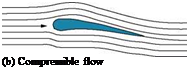by the existence of body in the flow field, the streamlines are more displaced in a compressible flow than in an incompressible flow, as shown in Figure 9.8, that is the disturbances introduced by an object are larger in compressible flow than in incompressible flow and they increase with the rise in Mach number. This is so because in compressible flow there is density decrease as the flow passes over the body due to acceleration, whereas in incompressible flow there is no change in density at all. That is to say, across the body there is a drop in density, and hence by streamtube area-velocity relation (Section 2.4, Reference 1), the streamtube area increases as the density decreases. At Mx = 1, this disturbance becomes infinitely large and this treatment is no longer valid.

(a) Incompressible flow

Figure 9.8 Aerofoil in an uniform flow.

Using Equation (9.87a), the perturbation velocity and the pressure coefficient may be expressed as follows:

дф _ 1 дф|пс

dx V/1—dxinc’

Therefore:

u inc

u = —, •

v/1-ML

Since the lift coefficient CL and pitching moment coefficient CM are integrals of CP, they can be expressed following Equation (9.87b) as:

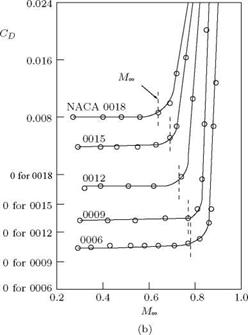
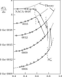
Variation of (a) lift-curve slope and (b) drag coefficient with Mach number (o-measured).

2. The ratio between aerodynamic coefficients in compressible and incompressible flows is also

1Л/1 – .

From Equations (9.87c) and (9.87f), we infer that the locations of aerodynamic center and center of pressure do not change with the freestream Mach number Mx, as they are ratios between CM and CL.

The theoretical lift-curve slope and drag coefficient from the Prandtl-Glauert rule and the measured CL and CD versus Mach number for symmetrical NACA-profiles of different thickness are shown in Figure 9.9.

From this figure it is seen that the thinner the aerofoil the better is the accuracy of the P-G rule. For 6% aerofoil there is good agreement up to MOT = 0.8; for 12% aerofoil also, the agreement is good up to Mx = 0.8; thus 12% may be taken as the limit of applicability of the Prandtl-Glauert (P-G) rule. For 15% aerofoil, there is good agreement up to MOT = 0.6. But above Mach 0.6, there is no more agreement. However, for supersonic aircraft the profiles used are very thin; so from a practical point of view, the P-G rule is very good even with the contradicting assumptions involved.

Beyond a certain Mach number, there is decrease in lift. This can be explained by Figure 9.9(b). There is sudden increase in drag when the local speed increases beyond sonic speed. This is because at sonic point on the profile, there is a X —shock which gives rise to separation of boundary layer, as shown in Figure 9.10.

The freestream Mach number which gives sonic velocity somewhere on the boundary is called critical Mach number M^. The critical Mach number decreases with increasing thickness ratio of profile. The P-G rule is valid only up to about M^.

Moo

From Section 9.8, it is seen that the governing equation for compressible flow is elliptic for subsonic flows (that is, for Mx < 1) and becomes hyperbolic for supersonic flows (that is, for > 1). This change in the nature of the partial differential equation, upon going from subsonic to supersonic flow, indicates the possibility of deriving similarity relationships between subsonic compressible flow and the corresponding incompressible flow, and the importance of Mach wave in a supersonic solution. In this chapter we shall derive an expression which relates the subsonic compressible flow past a certain profile to the incompressible flow past a second profile derived from the first principles through an affine transformation. Such an expression is called a similarity law.

If the governing equations of motion could be solved easily, the solution themselves would indicate quite clearly the nature of any similarities which might exist among members of a family of flow patterns. Then there is no need for a separate derivation of similarity laws.

But in the majority of situations, we are unable to solve the equations of motion. However, even though solutions are lacking, we may use our knowledge of the forms of the differential equations and the related boundary conditions to derive the similarity laws.

Pressure coefficient is the nondimensional difference between a local pressure and the freestream pressure. The idea of finding the velocity distribution is to find the pressure distribution and then integrate it to get lift, moment, and pressure drag. For three-dimensional flows, the pressure coefficient Cp given by (Equation (2.54) of Reference 1) is:

where M» and V» are the freestream Mach number and velocity, respectively, u, v and w are the x, y and z-components of perturbation velocity and y is the ratio of specific heats. Expanding the right-hand side of this equation binomially and neglecting the third and higher-order terms of the perturbation velocity components, we get:

For two-dimensional or planar bodies, the Cp simplifies further, resulting in:

This is a fundamental equation applicable to three-dimensional compressible (subsonic and supersonic) flows, as well as for low speed two-dimensional flows.

9.11.1 Bodies of Revolution

For bodies of revolution, by small perturbation assumption, we have u ^ У», but v and w are not negligible. Therefore, Equation (9.73) simplifies to:

u v2 + w2 C — —2 ‘

= 2 V V 2

V oo V ^

The above equation, which is in Cartesian coordinates, may also be expressed as:

„ u f v/l 2 Cp = -2^ – .

Combining Equations (9.72) and (9.75), we get:

where R is the expression for the body contour.

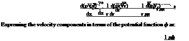
Fuselage of airplane, rocket shells, missile bodies and circular ducts are the few bodies of revolutions which are commonly used in practice. The general three-dimensional Cartesian equations can be used for these problems. But it is much simpler to use cylindrical polar coordinates than Cartesian coordi­nates. Cartesian coordinates are x, y, z and the corresponding velocity components are Vx, Vy, Vz. The cylindrical polar coordinates are x, r, в and the corresponding velocity components are Vx, Vr, Vg. For axisymmetric flows with cylindrical coordinates, the equations will be independent of в. Thus, mathe­matically, cylindrical coordinates reduce the problem to become two-dimensional. However, for flows which are not axially symmetric (e. g., missile at an angle of attack), в will be involved. The continuity equation in cylindrical coordinates is:

The potential Equation (9.50) can be written, in cylindrical polar coordinates, as:

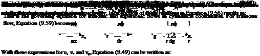
Also,

Equation (9.63) is the equation for axially symmetric transonic flows. All these equations are valid only for small perturbations, that is, for small values of angle of attack and angle of yaw (< 15°).

Conclusions

From the above discussions on potential flow theory for compressible flows, we can draw the following conclusions:

1. The small perturbation equations for subsonic and supersonic flows are linear, but for transonic flows the equation is nonlinear.

2. Subsonic and supersonic flow equations do not contain the specific heats ratio у, but transonic flow equation contains у. This shows that the results obtained for subsonic and supersonic flows, with small perturbation equations, can be applied to any gas, but this cannot be done for transonic flows.

3. All these equations are valid for slender bodies. This is true of rockets, missiles, etc.

4. These equations can also be applied to aerofoils, but not to bluff shapes like circular cylinder, etc.

5. For nonslender bodies, the flow can be calculated by using the original nonlinear equation.

9.9.1 Solution of Nonlinear Potential Equation

(i) Numerical methods.

The nonlinearity of Equation (9.49) makes it tedious to solve the equation analytically. However, solution for the equation can be obtained by numerical methods. But a numerical solution is not a general solution, and is valid only for a specific configuration of flow field with a fixed Mach number and specified geometry.

(ii) Transformation (Hodograph) methods.

When one velocity component is plotted against another velocity component, the resulting curve may be linear, whereas in the physical plane, the relation may be nonlinear. This method is used for solving certain transonic flow problems.

(iii)Similarity methods.

In these methods, the boundary conditions need to be specified for solving the equation. Detailed discussion of this method can be found in Chapter 6 on Similarity Methods.

9.5 Boundary Conditions

Examine the streamlines around an aerofoil kept in a flow field as shown in Figure 9.6.

In inviscid flow, the streamline near the boundary is similar to the body contour. The flow must satisfy the following boundary conditions (BCs).

Boundary condition 1 – Kinetic Bow condition

The flow velocity at all surface points are tangential on the body contour. The component of velocity normal to the body contour is zero.

Boundary condition 2

At z ^ ±x, perturbation velocities are zero or finite. The kinematic flow condition for the aerofoil shown in Figure 9.6, with small perturbation assumptions, may be written as follows.

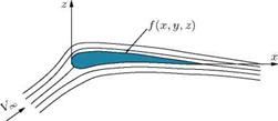
Body contour: f = f (x, y, z)

The velocity vector V at any point on the body is tangential to the surface. Therefore, on the surface of the aerofoil, (V • vf) = 0, that is:

where the subscript “c” refers to the body contour and (dz/dx) is the slope of the body, and u and v are the tangential and normal components of velocity, respectively. Expressing u and w as power series of z, we get:

u(x, z) = u(x, 0) + az + a2z2 + … w(x, z) = w(x, 0) + hiz + b2z2 + …

The coefficients a’s and h’s in these series are functions of x. If the body is sufficiently slender:

w(x, 0) _ ( dz^

Vx + u(x, 0) (dx ) C

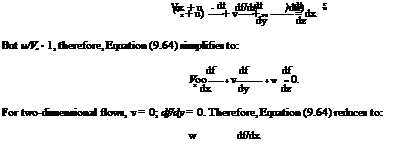
that is, for sufficiently slender bodies, it is not necessary to fulfill the boundary condition on the contour of the aerofoil. It is sufficient if the boundary condition on the x—axis of the body is satisfied, that is, on the axis of a body of revolution or the chord of an aerofoil. With u/Vx ^ 1, the above condition becomes:

that is, the condition is satisfied in the plane of the body. In Equations (9.67) and (9.68), the elevation of the body above the x—axis is neglected.

9.10.1 Bodies of Revolution

For bodies of revolution, the term 1 d (rvr) present in the continuity equation (9.54) becomes finite. Because of this term, the perturbations near the body become significant. Therefore, a power series for velocity components is not possible. However, we can apply the following approximation to express the perturbation velocity as a power series. For axisymmetric bodies:

From the above discussions, it may be summarized that the boundary conditions for this kind of problem are the following.

For two-dimensional (planar) bodies:

The general equation for compressible flows, namely Equation (9.40), can be simplified for flow past slender or planar bodies. Aerofoil, slender bodies of revolution and so on are typical examples for slender bodies. Bodies like wing, where one dimension is smaller than others, are called planar bodies. These bodies introduce small disturbances. The aerofoil contour becomes the stagnation streamline.

For the aerofoil shown in Figure 9.4, with the exception of nose region, the perturbation velocity w is small everywhere.

9.8.1 Small Perturbation Theory

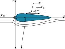
Assume that the velocity at any point in the flow field is given by the vector sum of the freestream velocity VOT along the x-axis, and the perturbation velocity components u, v and w along x, у and z-directions, respectively. Consider the flow around an aerofoil shown in Figure 9.4. The velocity components around the aerofoil are:

Vx = Vx, + u, Vy = v, Vz = w, (9.42)

where Vx, Vy, Vz are the main flow velocity components and u, v, w are the perturbation (disturbance) velocity components along x, у and z directions, respectively.

The small perturbation theory postulates that the perturbation velocities are small compared to the main velocity components, that is:

u < Уж, v < Уж, w < У

Therefore:

Ух« Уж, у, << Уж, V << Уж. (9.43*)

Now, consider a flow at small angle of attack or yaw as shown in Figure 9.5. Here:

Ух = Уж cos a + u, Уу = Уж sin a + v.

Since the angle of attack a is small, the above equations reduce to:

Ух = Уж + u, Уу = v.

Thus, Equation (9.42) can be used for this case also.

With Equation (9.42), linearization of Equation (9.40) gives:

(1 – И2)фхх + фуу + Фїї = 0, (9.44)

neglecting all higher order terms, where M is the local Mach number. Therefore, Equation (9.41) should be used in solving Equation (9.44).

a

The perturbation velocities may also be written in potential form, as follows: Let ф = фж + q>, where:

фж — : фхх —фжх$ + Фхх. . .

Therefore, ф may be called the disturbance (perturbation) potential and hence the perturbation velocity components are given by:

дф дф дф

u = —, v = —, w = —. дх dy dz

With the assumptions of small perturbation theory, Equation (9.41) can be expressed as:

a 2 , , u

— ) = – (y – ) Mж — аж ‘ V ж

(аж )2 — (■ – Y – «-і u )-‘.

Using Binomial theorem, (аж/а)2 can be expressed as:

( ^)! = 1 + (Y – 1) U M + °(m» I )

Substituting the above expression for (аж/а) in the equation:

M = (1 + u) (т) M~,

the relation between the local Mach number M and freestream Mach number Мж may be expressed as (neglecting small terms):

The combination of Equations (9.48) and (9.44) gives:

Equation (9.49) is a nonlinear equation and is valid for subsonic, transonic and supersonic flow under the framework of small perturbations with u ^ Уж, v ^ Уж and w ^ Уж. It is, however, not valid for hypersonic flow even for slender bodies (since u & Уж in the hypersonic flow regime). The equation is called the linearized potential Bow equation, though it is not linear.

Equation (9.49) may also be written as:

Further linearization is possible if:

With this condition Equation (9.50) results in:

This is the fundamental equation governing most of the compressible flow regime. Equation (9.52) is valid only when Equation (9.51) is valid and Equation (9.51) is valid only when the freestream Mach number Ml is sufficiently different from 1. Hence, Equation (9.51) is valid for subsonic and supersonic flows only. For transonic flows, Equation (9.49) can be used. For Ml & 1, Equation (9.49) reduces to:

The nonlinearity of Equation (9.53) makes transonic flow problems much more difficult than subsonic or supersonic flow problems.

Equation (9.52) is elliptic (that is, all terms are positive) for Ml < 1 and hyperbolic (that is, not all terms are positive) for Ml > 1. But in both the cases, the governing differential equation is linear. This is the advantage of Equation (9.52).

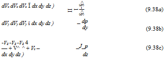
For a steady, inviscid, three-dimensional flow, by continuity equation:

v • (pV) = 0,

that is:

d(pVx) д(рУу) д(руг)

dx ду dz

Euler’s equations of motion (neglecting body forces) are:

P

P

P

For incompressible flows, the density p is a constant. Therefore, the above four equations are sufficient for solving the four unknowns Vx, Vy, Vz and p. But for compressible flows, p is also an unknown. Therefore, the unknowns are p, Vx, Vy, Vz and p. Hence, the additional equation, namely, the isentropic process equation, is used. That is, pjpY = constant is the additional equation used along with continuity and momentum equations.

Introducing the potential function ф, we have the velocity components as:

дф дф дф

Vx = І = фХ, Vy = дф = фУ, Vz = І = фz.

Equation (9.37) may also be written as:

From isentropic process relation, p = p(p). Hence:

because from Equation (9.38a):

( dVx dVx dVx ) dp

Vx —- + Vy —- + Vz—, —

^ dx y dy dz ) dp

Similarly:

But the velocity components and their derivatives in terms of potential function can be expressed as:

dVx dVy z

-x = фхх, – у = фуу, it = ф»

dVx – Vy – Vz

—- = фиУ, —– У = ф-к, —– = фzx-

ду xy dz yz dx zx

Therefore, in terms of potential function ф, the above equation can be expressed as:

t1 – a) ф“ + I1 – ал фуу + f1 – %)

This is the basic potential equation for compressible flow and it is nonlinear.

The difficulties associated with compressible flow stem from the fact that the basic equation is nonlinear. Hence the superposition of solutions is not valid. Further, in Equation (9.40) the local speed of sound ‘а is also a variable. By Equation (2.9e) of Reference 1, we have:

To solve a compressible flow problem, we have to solve Equation (9.40) using Equation (9.41), but this is not possible analytically. However, numerical solution is possible for given boundary conditions.

Consider two-dimensional, steady, inviscid flow in natural coordinates (l, n) such that l is along the streamline direction and n is perpendicular to the direction of the streamline. The advantage of using natural coordinate system – a coordinate system in which one coordinate is along the streamline direction and other normal to it – is that the flow velocity is always along the streamline direction and the velocity normal to streamline is zero.

Though this is a two-dimensional flow, we can apply one-dimensional analysis, by considering the portion between the two streamlines 1 and 2 (as shown in Figure 9.3) as a streamtube and taking the third dimension to be to.

Let us consider unit width in the third direction, for the present study. For this flow, the equation of continuity is:

The /-momentum equation can also be expressed as: dV dp pV— = —-. f dl dl The n-momentum equation is: dV = 0. But there will be centrifugal force acting in the n-direction. Therefore: pV2 _ dp R dn

(9.27)

(9.28)

The energy equation is:

V2 h + — = h0.

(9.29)

The relation between the entropy and enthalpy can be expressed as [1]:

Differentiation of Equation (9.29) gives dh + VdV = dh0. Therefore, the entropy equation becomes:

Tds = — V dV + — ) + dh0. p

This equation can be split as follows: (i)

ds! dV 1 dp dl dl p dl I

ds f dV 1 dp dh0 dn у dn p dn J dn Introducing dp/dl from Equation (9.27) and dp/dn from Equation (9.28) into the above two equations, we get:

ds T — = 0 dl ds (dV V dh0 T — = – V—————– + —-. dn V dn R ) dn

But, (R — = z is the vorticity of the flow. Therefore:

This is known as Crocco’s theorem for two-dimensional flows. From this, it is seen that the rotation depends on the rate of change of entropy and stagnation enthalpy normal to the streamlines.

Crocco’s theorem essentially relates entropy gradients to vorticity, in steady, frictionless, nonconduct­ing, adiabatic flows. In this form, Crocco’s equation shows that if entropy (s) is a constant, the vorticity (Z) must be zero. Likewise, if vorticity Z is zero, the entropy gradient in the direction normal to the streamline (ds/dn) must be zero, implying that the entropy (s) is a constant. That is, isentropic flows are irrotational andirrotational flows are isentropic. This result is true, in general, only for steady flows of inviscid fluids in which there are no body forces acting and the stagnation enthalpy is a constant.

From Equation (9.30a) it is seen that the entropy does not change along a streamline. Also, Equation (9.30Z>) shows how entropy varies normal to the streamlines.

The circulation is:

By Stokes theorem, the vorticity Z is given by:

(9.33)

dV^_ 9Vy dy dz J dVx_dVz dz dx J dVy _dVx dx dy J

where Zx, Zy, Zz are the vorticity components. The two conditions that are necessary for a frictionless flow to be isentropic throughout are:

1. h0 = constant, throughout the flow.

2. Z = 0, throughout the flow.

From Equation (9.33), Z = 0 for irrotational flow. That is, if a frictionless flow is to be isentropic, the total enthalpy should be constant throughout and the flow should be irrotational.

It is usual to write Equation (9.33) as follows:

Z = (V x V)

i j к

_ d d d

dx dy dz

( V V V (

Vx Vy Vz

When Z = 0

Since h0 = constant, T0 = constant (perfect gas). For this type of flow, we can show that:

T ds RT0 dp 0

V dn V p0 dn

From Equation (9.34), it is seen that in an irrotational flow (that is, with Z = 0), stagnation pressure does not change normal to the streamlines. Even when there is a shock in the flow field, p0 changes along the streamlines at the shock, but does not change normal to the streamlines.

Let h0 = constant (isoenergic flow). Then Equation (9.31) can be written in vector form as:

where grad s stands for increase of entropy s in the n-direction. For a steady, inviscid and isoenergic flow:

T grad s + V x curl V = 0

V x curl V =-Tgrads. (9.35b)

If s = constant, V x curl V = 0. This implies that (a) the flow is irrotational, that is, curl V = 0, or (b) V is parallel to curl V.

Irrotational flow

For irrotational flows (curl V = 0), a potential function ф exists such that:

(9.36)

On expanding Equation (9.36), we have:

дф дф

iVx + jVy + kVz = ідф + jJL +

dx dy

Therefore, the velocity components are given by:

дф	V= дф y dy’
dx

The advantage of introducing ф is that the three unknowns Vx, Vy and Vz in a general three-dimensional flow are reduced to a single unknown ф. With ф, the irrotationality conditions defined by Equation (9.33) may be expressed as follows:

дVz

Zx = IT дy

д дф д

д^ д^ J дz

Also, the incompressible continuity equation v • V = 0 becomes:

or

v2ф = 0 •

This is Laplace’s equation. With the introduction of ф, the three equations of motion can be replaced, at least for incompressible flow, by one Laplace equation, which is a linear equation.

9.6.1 Basic Solutions of Laplace’s Equation

We know from our basic studies on fluid flows [2] that:

1. For uniform flow (towards positive x-direction), the potential function is:

ф = V» x.

2. For a source of strength Q, the potential function is:

, Q ,

ф = — ln r.

2n

3. For a doublet of strength p. (issuing in negative x-direction), the potential function is:

p. cos в

ф = ——– •

r

4. For a potential (free) vortex (counterclockwise) with circulation Г, the potential function is:

Г

ф = ^в.

2п