Category Aerodynamic measurements

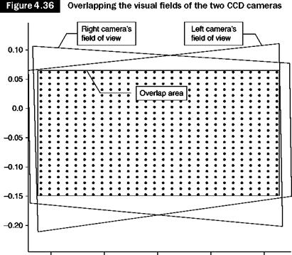
The 3D PIV uses the stereoscopic principle to identify the three components of speed in a flat section of the flow field determined by the laser light sheet. The 3D (Dx, Dy, Dz) displacement is estimated by a couple of 2D (Dx, Dy) displacements as seen by the left and right cameras (Figure 4.35). The greater the angle between the two cameras, the more accurate is the determination of the displacement Dz.

The 3D processing requires a numerical model that describes how objects in space are seen by the CCD camera. The parameters of the numerical model are obtained from a preliminary calibration of the

camera framing markers whose position is known: it serves to identify a common coordinate system for the two cameras.

Obviously, the 3D assessment is only possible within the area covered by both cameras. (Figure 4.36). Because of the perspective distortion, each camera covers a region of the trapezoidal plate light. Careful alignment to maximize the overlap area is required.

The stereoscopic measurement begins by processing the simultaneous images produced by two cameras. Two 2D vector maps are obtained that describe the flow field as seen by each of the two cameras. Using the calibration function with the parameters obtained during calibration of the camera, the points of the interrogation grid are reported from the plane of the light sheet on the left and right image planes (planes of the CCDs). With the 2D displacement seen by both cameras and estimated at the same point of the physical space, the 3D displacement of the particle can be calculated by solving the equations obtained in calibration.

When the light sheet is observed at an angle different from 90°, the image plane of the camera, the plane of the CCD, must be rotated as required to properly focus the entire field of view of the camera. The planes of the image, of the lens and of the object must intersect along a common line in order to obtain a properly focused image. This is called the Scheimpflug condition.

Unlike the laser techniques described above, LDA and L2F, which provide velocity measurements at one point, PIV allows the examination of a whole section of the flow field and thus enables simultaneous measurement at different points, that is an essential requirement in unsteady motions. Usually two components of velocity are measured, but using a stereoscopic approach it is possible to obtain three components. The use of modern charged-couple device (CCD) cameras and dedicated computing
hardware permits velocity and vorticity maps in real time to be obtained, of the same type as those obtained in computational fluid dynamics (CFD) with the large eddy simulation technique.

4.5.1 PIV for studies of 2D fields

The test section is illuminated by a sheet of laser light produced by a cylindrical lens (Figure 4.31). This produces an image of the illuminated area on the matrix of pixels (typically 1k x 1k) of a CCD camera. To maximize the amount of light that reaches the camera, it should be placed in the direction of forward scatter, but the visual field would be reduced, the location chosen is usually normal to the direction of motion.

In the PIV, velocity vectors are determined by measuring the dis­placements of particles between two consecutive images of the stream:

Dt

Diagram of a PIV apparatus for 2D fields

To find the individual velocity vector, the images are divided into interrogation areas or sections or windows (Figure 4.32), in which it is assumed that all particles have the same speed. In order to obtain a significant measure, 10 to 25 particles must be contained in each area. The lateral size of the interrogation area, dIA, must be chosen, depending on the size of the structure of the stream that must be investigated. One way to express this is to state that the velocity gradient is negligible inside the interrogation area, for example, it must be:

V – V

^ minAt< 5%

dIA

The maximum measurable speed is limited by the particles that exceed the boundaries of the interrogation area in the time that elapses between the two laser pulses. The condition can be imposed:

The measurement volume can be defined once the size of the interrogation area and the thickness of the light sheet are known.

There are two possible procedures:

■ double-exposure image

■ two separate images.

The first procedure allows the movement of particles to be viewed and the structures present in the stream to be highlighted. To each area of interrogation a technique of autocorrelation is applied: denoting by

I(x, y) the intensity of light scattered by the particles, and by Z and h the shifts in the directions x and y, the convolution integral is applied in the interrogation area and the maximums are found:

R (£, n) = J J I(x, y) * I(x – £, y – n) dxdy

The absolute maximum identifies the null displacement, the overlapping of individual particles. The next maximum identifies the distance in the two directions between two consecutive positions of the particle. This procedure therefore does not determine the direction of the speed so it is not applicable in vortical zones where there are inversions of velocity.

To use the second procedure, it is necessary to use a CCD camera capable of capturing on separate frames the images produced by laser pulses. Once a couple of pulses are recorded, the areas of interrogation of both frames are cross-correlated pixel by pixel. In an interrogation window of M x N pixels (Figure 4.33), the common particle displacement can be calculated using the algorithm of cross-correlation:

M N

C(Ax Ay) =Y7LI1 (Ji j) * I2 ( – j – Dy)

,=i j=1

where Dx and Ay are possible displacements obviously limited by the condition that the particles do not exceed the boundaries of the window. The correlation produces a peak signal that identifies the common particle displacement Ax, Ay). Accurate measurement of displacement, and therefore of the speed, is obtained with a sub-pixel interpolation.

A map of the velocity vector in the whole investigated area is obtained by repeating the cross-correlation for each interrogation area on the two

frames (Figure 4.34). In the same figure the corresponding map of vorticity is shown calculated from:

_dv-du Ю~ dx dy

If a flow is periodic, it is necessary to correlate the measured velocity with the phase of the periodic phenomenon, e. g. in measurements in turbo engines, the measurement volume sweeps a path in the circumferential row of rotating blades, thus the flow between two blades is present cyclically with a frequency that depends on the speed of rotation and the number of blades. A synchronizer, working like an electronic shaft position encoder detects a pulse generated from the shaft itself. The frequency of the input signal (one lap) is multiplied by the number of blades to generate a pulse per blade (frequency of the blades).

If measurements are made between the blades of a turbo engine in motion, the laser beam must be instantly shut down, in order to pre­vent strong reflections of the laser beam on the blades. This mode of operation improves the signal to noise ratio as the photocathodes of the photomultiplier are restored during periods of absence of laser light.

If a turbine disk with 30 blades is running at 10,000 rpm, laser beams encounter a blade 5,000 times a second: no mechanical shutter is capable of such a performance. A Bragg cell is then used which, as already stated, consists of a transparent crystal which is excited by a piezoelectric transducer connected to a high frequency generator; by applying an alternate current to the transducer, a train of acoustic waves is generated inside the crystal, that produces a periodic variation of the refractive index of the crystal which, in turn, generates the periodic diffraction of the laser beam. The outgoing beam oscillates with the frequency of the transducer in turn generating a beam of zero order (non-deviated), beams of the first order, second, and so on (Figure 4.30).

If the piezoelectric transducer is not excited, the incoming beam undergoes no deviation (zero-order beam only exiting the crystal), and is thus interrupted by the optical stop; the Bragg cell and the stop are adjusted so that, with the transducer excited, the beam of the first order is able to exit the hole in the optical stop with a frequency equal to that of the blades.

The output signals from the photomultipliers are images of the intensity profile of the focal volume with the addition of noise in varying amounts: accurate signal processing techniques are needed in order to achieve a good resolution of flight time.

The signal is sent to an amplifier at fixed gain and then to an adjustable low-pass filter, which allows the elimination of high frequency noise and thus increases the signal to noise ratio, an additional amplifier sends the signal to a constant fraction discriminator (CFD) unit. This emits a pulse output when the signal exceeds a predetermined fraction of its maximum value, the output signal is in this way independent of the size of the input signal. If this amplitude exceeds a trigger level, which may occur when a particle is too large and therefore not indicative of the stream velocity, the CFD discards the measure.

The start impulse enables a precise current to charge a capacitor, whose voltage rises according to a characteristic ramp law, the stop impulse interrupts the charge, so a voltage signal is generated proportional to the time interval between the two pulses (time of flight).

Each of the two ideal measurement volumes can be defined as that zone of the focus contained within the surface on which the light intensity is equal to 1/e2 of its maximum value: if the intensity distribution of a laser beam is Gaussian, the surface will be an ellipsoid (Figure 4.29a). The real measurement volume is the undefined region from which the scattered light is projected onto each photomultiplier.

To properly define the boundaries of the measurement volume, the scattered light coming back towards the detectors is filtered through calibrated holes that allow only the passage of light from a narrow

Measurement volume of L2F: (a) in the plane of the laser beams; (b) in the normal plane

(a)

(b) region, which is the real measurement volume. The ability to operate on the signal, setting the threshold level and allowing the passage only to signals of certain characteristics, increases the definition of the measurement zone, making it very close to the theoretical one, for example, very weak signals are typical of light scattered by particles crossing laser beams in areas different from the focus.

The diameter d of the spots in the area of measurement is about 10 pm, the distance s between the two is about 102 pm (remember that the size of the spot of an LDA is of the order of 1 mm). If the distance l » 2s, the angle ф shown in Figure 4.29a is 45°. Note in Figure 4.29b that the finite diameter of the spot induces uncertainty about the exact distance traveled by the particle. Figure 4.29b shows that start and stop pulses can be generated by particles traveling either according to the line joining the axes of two laser beams or, at worst, according to the tangent at the bottom left and top right of the beams. The maximum relative error is:

є =——– = 1 – cos I sin 1

s

The error decreases as the ratio s/d. On the other hand, the probability of two related events decreases when this ratio increases.

As the two focal volumes are thousands of times brighter than the measuring volume of a LDA of equal power, the L2F can be easily used in the back-scatter configuration, which allows placement into a single hardware of both emission and receiving optics, in this way there are no alignment problems since the vibrations are transmitted evenly to both elements.

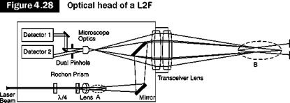Figure 4.28 shows a typical L2F optical head: it includes two photomultipliers (detectors 1 and 2), a beam-splitter (Rochon prism), a

1/4, the transceiver lens, and mirrors and lenses necessary to focus the laser beams and to create in the measurement of zone B the image of the two foci produced in zone A.

The laser light, monochromatic and linearly polarized, passes through a 1/4, i. e. a filter that slows and overlaps the incident waves; by the superimposition of two electromagnetic waves having the same form but out of phase by 90°, a quarter of wavelength, a circularly polarized wave is created.

The Rochon prism separates the laser beam into two beams of equal intensity: one emerges essentially not deflected, the other with a small angle with respect to the optical axis: a lens therefore focuses the two beams into two distinct focus; their distance can be changed using Rochon prisms with different angles of divergence.

The transceiver consists of two collimator lenses without spherical aberration flanked on all openings; the front collimator is interchangeable to allow for changes in working distance. The particles that pass through the focal volume scatter the laser light in all directions. The transceiver lens captures the back-scattered light and focuses it on a double pinhole that acts as a filter for the light background as in it passes only the light from the focal volume. Two broadband photomultiplier tubes convert the light pulses of start and stop into electrical pulses.

The change in the direction of measurement in the plane perpendicular to the optical axis is obtained by rotating around its axis the Rochon prism, the double pinhole optics and other stops, in this way, the off-axis focus is turned around the central focus that remains fixed in space (Figure 4.25). This fact justifies the presence of the 1/4, because the circularly polarized beam prevents variations of the light intensity of the beam when the prism rotates.

4.4.1 Principle of operation

In the L2F, also known as a laser transit anemometer (LTA), the fluid stream velocity is obtained, by its definition, by measuring the time taken by a particle driven by the fluid to travel the distance between two light targets generated by two highly focused laser beams. The idea dates back to 1968 when it was introduced by D. H. Thompson. However, a tracer particle fluid velocity meter was only suitable for measuring velocities of the order of 20 m/s in the absence of turbulence. In 1973, Tanner, Schodl and Lading introduced new methods of analysis that allowed the extension of the measurements even at moderately turbulent flows (turbulence intensity up to 30%) and at supersonic speeds.

Figure 4.23 shows a particle traveling a trajectory normal to the axes of both beams. A signal of start from light scattered by a particle crossing the first focus activates a timer and when the particle crosses the second focus a signal of stop is sent to the timer. The flight time is the time interval between two pulses of start and stop for the same particle (correlated pulses).

If in the measurement zone there are two separate particles and/or the direction of velocity is not normal to both axes (Figure 4.24), the start and stop pulses are generated by different particles. The time interval measured has no correlation with particle velocity, i. e. random pulses.

With a single measurement it is not possible to decide whether the measured time interval is random or if it is the flight time of a particle. Making a significant number of measures of time intervals the data with no correlation are averaged as a background noise while the correlated data will tend to be distributed according to a quasi-Gaussian curve like those in Figure 4.9.

To locate the direction of the velocity in the plane perpendicular to the optical axis, it is necessary to accumulate histograms in all directions of the plane; this is done by rotating one beam around the other (Figure 4.25). Histograms taken at different angular positions produce a 2D histogram, speed-direction. If the velocity vector lies in the chosen plane (2D flow), the histogram shows a peak and both the most likely value of the speed and of the direction of the velocity vector can be read from it (Figure 4.26).

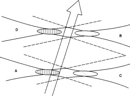
If the flow is not in the plane perpendicular to the optical system, the number of correlated impulses falls. The 3D L2F utilizes this effect to obtain velocity information in three dimensions. Using two colors of a laser, a pair of focal volumes is generated for each beam displaced along the optical axis, as shown in Figure 4.27. The system simultaneously measures the times of flight from A to B and from C to D: the distance of the direction of the velocity is obtained by the ratio between the number of data in these two channels.

From the mathematical point of view, the easiest way to determine the frequencies contained in a signal is to convert the signal in the frequency domain through Fourier transforms. A simple way to implement the

Errors in fixed time counting techniques

Gate time matched to low velocity signals

Fourier transform in the hardware of a computer, i. e. in discrete form on a limited number of samples, is called the FFT (fast Fourier transform).

The signal from the photomultiplier is digitized in an A-D converter that will take samples whose number must be chosen according to the length of the signal: 8, 16, 32 or 64 with a sampling frequency corresponding to the selected bandwidth. The procedure is applied to all signals coming in; only those due to the passage of particles in the control volume must be selected, therefore the times of arrival and departure of the particle in the volume are recorded and the process of storage signals is started and ended.

A power spectrum is calculated by the equation:

k=-N, – N+ 1,…,N-1

where N (= number of samples) may have the values 8, 16, 32 or 64.

A post-processor estimates the Doppler frequency using a parabolic interpolation of the measured spectrum. Inspection of the spectrum is also carried out: the measure is discarded if a peak does not appear in the frequency spectrum. Doppler frequencies of the measures that are accepted are sent to the output buffer along with the times of arrival and residence of the particle in the control volume.

The FFT processors are very accurate. With them an experienced user can achieve results not available with other types of processors: signals with low SNR values or even completely immersed in noise can be handled; for this reason the FFT processors are the most suitable for research applications.

The method of correlation is a technique well known from radar technology. Part of the Doppler signal is delayed by a known time t: this is equivalent to adding a phase equal to the frequency multiplied by t. The two signals, the original and the delayed one are compared in a cross-correlator which measures the phase difference from which, dividing by the known delay, the frequency is obtained. Correlators are simple to use and, because of their low cost, are the preferred choice in industrial applications.

4.3.7.3 Period counters

When the number of signals per unit time is low, a high speed analog – digital converter can be used. The output signal of the photomultiplier is amplified, sent to a band-pass filter, digitized by the analog-digital converter and sent to a computer.

If the signal has only one frequency, the time between two zeros, which represent crossings of dark fringes (Figure 4.12), is the period. In order to minimize measurement error, the meter is programmed to count a number of zeros, and the period is obtained by the measured time divided by the number of zeros.

The computer checks the validity of each signal by comparing the time intervals between successive zeros (typically time intervals of 5 and 8 zeros). Only if these times give equal periods within the limits chosen, and only if the global number of zeros is not much smaller than the number of fringes contained in the control volume, is the signal accepted as valid. With these controls it is possible to detect signals disturbed by noise or signals generated by highly oblique particles passing through the control volume or those produced by two particles crossing this volume simultaneously.

Note that periods are measured and not frequencies (number of zeros in a fixed time); Figure 4.22 clearly shows the kind of errors made when measuring the frequency: if the measurement time is too small compared to the duration of the signal, few oscillations and fractions are included in it and therefore the error is large; if the measuring time is larger than the duration of the signal, the error is made of dividing the number of zeros for the gate time, which also includes a part when the signal is absent. As the length of the signal depends on the speed of the particle and the direction in which it crosses the measuring volume, the fixed time counting technique could only be used in quasi-stationary streams.

The period counter was the second system used in commercial anemometers, after the frequency tracker. Both systems are currently used for simple educational applications.

The filter has a window whose center frequency can be changed continuously. The bandwidth of the filter is critical: if the bandwidth is very narrow, there are many signals rejections and to build a good probability curve it is necessary to stay for a long time on each frequency; if the band is broadened, the precision of the measure decreases. This measuring system is very effective, but unfortunately highly inaccurate and relatively slow. It can be considered an excellent tool for tuning and diagnosis of the initial motion, but this is not the system to be chosen for routine measurements.

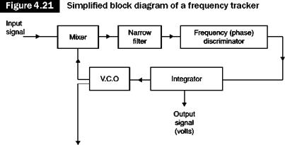
4.3.7.2 Frequency tracker

This measurement system was the first to be sold in complete systems anemometers. The working principle is illustrated in the block diagram of Figure 4.21: the input signal is mixed with the signal from an oscillator

whose frequency is a function of voltage applied to its input (voltage controlled oscillator, VCO). The two overlapping signals pass through the narrow filter and are directed to a frequency or phase discriminator, which works by comparing the phases of the two signals and that, through an integrator, generates an output signal in the form of a voltage, proportional to the difference in frequency, that is sent to the VCO. The output frequency of the VCO is then adjusted to remove this difference and is therefore a measure of the Doppler frequency.

This is a slave filter, which adapts automatically to the frequency of the signal. To use the frequency tracker properly, the signal should be continuous (very large concentration of particles). The problem that the signals are discrete is solved by a simple form of memory that allows, when the signal is not present, the oscillation frequency of the VCO to be set on the last reading. The typical problem of this system is that it fails to follow the fluctuations of turbulence beyond a certain limit value, the theoretical maximum permissible intensity of turbulence for a frequency tracker is 0.33.