Our heavyweight helicopter equal in the world does not have
In Rostov started production of the most load-lifting rotary-wing car The Russian holding «Helicopt[...]

Everything about aircrafts and helicopters. News and events in aviation worldwide. Civil, transportation, military helicopters and airplanes.

Everything about aircrafts and helicopters. News and events in aviation worldwide. Civil, transportation, military helicopters and airplanes.

Everything about aircrafts and helicopters. News and events in aviation worldwide. Civil, transportation, military helicopters and airplanes.

Everything about aircrafts and helicopters. News and events in aviation worldwide. Civil, transportation, military helicopters and airplanes.


The power-thrust relationship for level flight was derived in Chapter 5 and is given in idealized form in Equation 5.70, or with empirical constants incorporated in Equation 5.71. Generally we assume the latter form to be the more suitable for practical use and indeed to be adequate for most preliminary performance calculation. The equation shows the power coefficient to be the linear sum of separate terms representing, respectively, the induced power (rotor lift dependent), profile power (blade section drag dependent) and parasite power (fuselage drag dependent). It is in effect an energy equation, in which each term represents a separately identifiable sink of energy, and might have been calculated directly as such. In dimensional terms we have:
in which VT is the rotor tip speed, V the forward flight speed and f the fuselage-equivalent flat plate area, defined in Equation 5.88. The induced velocity Vi is given according to momentum theory by Equation 5.3; however, if we simplify the situation by assuming the rotor disc tilt is very small, Equation 5.3 can be rewritten as:
![]() T 1
T 1
Vi = 2pA ffiTVf
where VZ is neglected as small order compared with Vi and VX becomes V. The solution of (7.10) is given by:
Allowances should be added for tail rotor power and power to transmission and accessories: collecting these together in a miscellaneous item, the total is perhaps 15% of P at V = 0
|
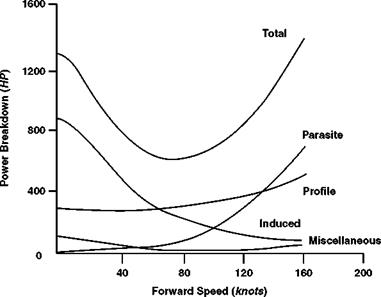
Figure 7.3 Typical power breakdown for forward level flight |
(Section 7.2) and half this, say 8%, at high speed. Otherwise, if the evidence is available, the items may be assessed separately. The thrust T may be assumed equal to the aircraft weight W for all forward speeds above 5 m/s (10 knots) although at the highest speeds, the fuselage drag needs careful attention.
A typical breakdown of the total power as a function of flight speed is shown in Figure 7.3.
Induced power dominates the hover but makes only a small contribution in the upper half of the speed range. Profile power rises only slowly with speed unless and until the compressibility drag rise begins to be shown at high speed. Parasite power, zero in the hover, increases as V3 and is the largest component at high speed, contributing about half the total. As a result of these variations the total power has a typical ‘bucket’ shape, high in the hover, falling to a minimum at moderate speed and rising rapidly at high speed to levels above the hover value. Except at high speed, therefore, the helicopter uses less power in forward flight than in hover.
Charts are a useful aid for rapid performance calculation. If power is expressed as P/d, where d is the relative air density at altitude, a power carpet can be constructed giving the variation of P/d with W/d and V. Figures 7.4a and b show an example, in which for convenience the carpet is presented in two parts, covering the low – and high-speed ranges. When weight, speed and density are known, the power required for level flight is read off directly.
The above is a relatively simple analysis of helicopter performance. The Appendix contains a fuller description of power prediction, the associated fuel consumption and mission analysis.
The formula relating thrust and power in vertical flight, according to blade element theory, was derived in Equation 3.54. The power required is the sum of induced power, related to blade lift, and profile power, related to blade drag. Converting to dimensional terms the equation is:
1 ,
P = ki(VC + Vi)T + 8 CD0MbVT (7.1)
where in the induced term, using momentum theory as in Equation 2.28, one may write:
If in Equation 7.1 the thrust is expressed in N, velocities in m/s, area in m2 and air density in kg/m3, the power is then in W or, when divided by 1000, in kW. Using imperial units, thrust in lb, velocities in ft/sec, area in ft2 and density in slugs/ft3 lead to a power in lb ft/sec or, on dividing by 550, to HP.
To make a performance assessment, Equation 7.1 is used to calculate separately the power requirements of main and tail rotors. For the latter, VC disappears and the level of thrust needed is such as to balance the main rotor torque in hover; this requires an evaluation of hover trim, based on the simple equation:
T • / = Q (7.3)
where Q is the main rotor torque and / is the moment arm from the tail rotor shaft perpendicular to the main rotor shaft. The tail rotor power may be 10-15% of main rotor power. To these two are added allowances for transmission loss and auxiliary drives, perhaps a further 5%. This leads to a total power requirement, Preq say, at the main shaft, for a nominated level of main rotor thrust or vehicle weight. The power available, Pav say, is ascertained from engine data, debited for installation loss. Comparing the two powers determines the weight capability in hover, out of ground effect (OGE), under given ambient conditions. The corresponding capability in ground effect (IGE) can be deduced using a semi-empirical relationship such as Equation 2.64. The aircraft ceiling in vertical flight is obtained by matching Preq and Pav for nominated weights and atmospheric conditions.
|
kiVc, ki /V2, 2T ~ + 2 V Vc + ГА |
|
VC(2—ki) + kiJ VC + 4V0 |
 |
|
In order to understand the sensitivity of power in climb to the climb rate, we recall Equation 2.27:
 |
|||
from which we obtain, after partial differentiation with respect to Vc:
where the overbar is used, as in Chapter 2, to denote normalization with respect to V0 and the derivative is related to small increments in power and climb rate.
If this argument is examined in reverse, we have an equation which relates the climb rate achievable for a given excess of power.
 |
||||
Equation 7.7 now becomes:
![]() climb rate factor
climb rate factor
where the thrust is assumed to be equal to the aircraft weight in an equilibrium state. The kD factor is applied to the thrust to take account of the fuselage download increased in the climb.
 |
Taking kj to be 1.15 and kD to be 1.025, the term in braces in Equation 7.8 is plotted in Figure 7.2.
As the climb rate increases, the climb rate factor term drops from a value of approximately 2 in the hover to approximately 1 at a high climb rate. This is because, as the helicopter climbs away from hover, the climb causes a fall in the value of downwash, saving power which will contribute to that available from the engine(s). As the climb rate increases, the downwash will reduce to a very small value so this beneficial effect is lost and the engine power surplus is all that is available to generate a climb velocity. The two-to-one variation in factor between a zero climb rate and a high climb rate (say 6000 ft/min) is typical. Stepniewski and Keys (Vol. II, p. 55) suggest a linear variation between the two extremes. It should be borne in mind, however, that at low rates of either climb or descent, vertical movements of the tip vortices relative to the disc plane are liable to change the power relationships in ways which cannot be reflected by momentum theory and which are such that the power relative to that in hover is actually decreased initially in climb and increased initially in descent. These effects, which have been pointed out by Prouty [1], were mentioned in Chapter 2. Obviously in such situations Equation 7.4 and the deductions from it do not apply.
7.1 Introduction
The preceding chapters have been mostly concerned with establishing the aerodynamic characteristics of the helicopter main rotor. We turn now to considerations of the helicopter as a total vehicle. The assessment of helicopter performance, like that of a fixed-wing aircraft, is at bottom a matter of comparing the power required with that available, in order to determine whether a particular flight task is feasible. The number of different performance calculations that can be made for a particular aircraft is of course unlimited, but aircraft specification sets the scene in allowing meaningful limits to be prescribed. A typical specification for a new or updated helicopter might contain the following requirements, exclusive of emergency operations such as personnel rescue and life saving:
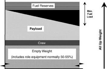
• Prescribed missions, such as a hover role, a payload/range task or a patrol/loiter task. More than one are likely to be called for. A mission specification leads to a weight determination for payload plus fuel and thence to an all-up weight, in the standard fashion illustrated in Figure 7.1.
• Some specific atmosphere-related requirements, for example the ability to perform the mission at standard (ISA) temperature plus, say, 15°; the ability to perform a reduced mission at altitude; the ability to fly at a particular cruise speed.
• Specified safety requirements to allow for an engine failure.
• Specified environmental operating conditions, such as to and from ships or oil rigs.
• Prescribed dimensional constraints for stowage, air portability and so on.
• Possibly a prescribed power plant.
Calculations at the flexible design stage are only a beginning; as a design matures, more will be needed to check estimates against actual performance, find ways out of unexpected difficulties, or enhance achievement in line with fresh objectives. (One is effectively zeroing in on the details.)
Generally, in a calculation of achievable or required performance, the principal characteristics to be evaluated are:
1. Power needed in hover.
2. Power needed in forward flight.
Basic Helicopter Aerodynamics, Third Edition. John Seddon and Simon Newman. © 2011 John Wiley & Sons, Ltd. Published 2011 by John Wiley & Sons, Ltd.
|
Figure 7.1 Determination of all-up weight for prescribed mission |
3. Envelope of thrust limitations imposed by retreating-blade stall and advancing-blade
compressibility drag rise.
The following sections concentrate on these aspects, using simple analytical formulae, mostly already derived. Item 3 must always be kept under review because the flight envelope so defined often lies inside the power limits and is thus the determining factor on level flight speed and manoeuvring capability.
A brief descriptive section is included on more accurate performance estimation using numerical methods. The chapter concludes with three numerical examples: the first concerns a practical achievement from advanced aerodynamics; the others are hypothetical, relating to directions in which advanced aerodynamics may lead in the future.
To complete this chapter we turn from research topics to the practical problem of determining the aerodynamic design of a rotor for a new helicopter project as shown in Figure 6.39.
A step-by-step process enables the designer to take into account the many and varied factors that influence their choice – aircraft specification, limitations in hover and at high forward speed, engine characteristics at various ratings, vibratory loads, flyover noise and so on. The following exposition comes from an unpublished instructional document kindly supplied by Westland Helicopters.
The basic requirement is assumed to be for a helicopter of moderate size, payload and range, with good manoeuvrability, robustness and reliability. The maximum flight speed is to be at least 80 m/s and a good high-temperature altitude performance is required, stipulated as 1200 m at ISA + 28 K. Prior to determining the rotor configuration, a general study of payload and range diagrams, in relation to the intended roles, leads to a choice of all-up weight, namely 4100 kg. Empty weight is set at 55% of this value, leaving 45% disposable weight, of which it is assumed one-half can be devoted to fuel and crew. Consideration of various engine options follows and a choice is made of a pair of engines having a continuous power rating at sea level ISA of 560 kW each, with take-off and contingency ratings to match. Experience naturally plays a large part in the making of these choices, as indeed it does throughout the design process.
First choice for the rotor is the tip speed: this is influenced by the factors shown in Figure 6.40. The tip Mach number in hover is one possible limitation. Allowing a margin for the fact that in high-speed forward flight a blade at the front or rear of the disc will be close to the same Mach number as in hover but at a higher lift coefficient, corresponding to the greater power required, the hover tip speed limit is set at Mach 0.69 (235 m/s). On the advancing tip in forward flight the lift coefficient is low and the Mach number limit can be between 0.8 and 0.9; recognizing that an advanced blade section will be used, the limit is set at 0.88. Flyover noise is largely a function of advancing tip Mach number and may come into this consideration. High
 Aircraft Specification
Engine
Characteristics
Vibratory Loads
 High Speed Limitations
Figure 6.39 Typical helicopter design constraints
advance ratio brings on rotor vibratory loads and hence fuselage vibration, so a limiting m for normal maximum speed is set at 0.4. Lastly the maximum speed specified is at least 80 m/s. It is seen that the satisfaction of these requirements constrains the rotor tip speed to about 215 m/s, the targeted maximum flight speed being 160 knots (82 m/s).
Next to be decided is the blade area. The area required increases as design speed increases, because the retreating blade operates at decreasing relative speed while its lift coefficient is stall limited. The non-dimensional thrust coefficient CT/s is limited as shown in Figure 6.41a – see Equation 3.45. Writing:
![]() W pR 1 pA(OR)2 Nc
W pR 1 pA(OR)2 Nc
![]()
 |
W
I 2
pNcR(OR)2
we have for the total blade area NcR:
From a knowledge of tip speed (OR) and aircraft weight the blade area diagram, Figure 6.41b, is constructed. The design maximum speed then corresponds to a total blade area of 10 m2. Note that use of the advanced blade section results in about 10% saving in blade area, which translates directly into rotor overall weight.
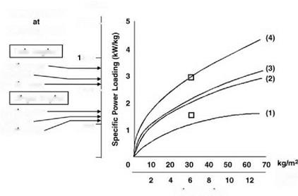
Choice of the rotor radius requires a study of engine performance. For the vertical axis in Figure 6.42, specific power loading (kW/kg) from the engine data is translated into actual power in W for the 4100 kg helicopter. Both twin-engine and single-engine values are shown, in each case for take-off, continuous and contingency ratings. Curves of power required for various hover conditions are plotted in terms of disc loading (kg/m2) on the established basis
(b)
 |
Determination of Blade Area
(Chapter 2) that induced power is proportional to the square root of disc loading. The four curves shown, reading from the lowest upwards, are:
(1) ideal induced power at sea level ISA, given by:
o being the disc loading;
 Disc Loading
Figure 6.42 Determination of rotor radius for new rotor design
(2) actual total power at sea-level ISA, scaled up from induced power to include blade profile power, tail rotor power, transmission loss, power to auxiliaries and an allowance for excess of thrust over weight caused by downwash on the fuselage;
(3) actual total power calculated for 1200 m altitude at ISA + 28°K;
(4) total power at sea level necessary to meet the requirement at (3), taking into account the decrease of engine power with increasing altitude and temperature.
A design point for disc loading can now be read off corresponding to the twin-engine take-off power rating (or using the contingency rating if preferred). From disc loading the blade radius follows, since:
![]() _ W _ W
_ W _ W
~ 1 ~ PR2
Hence:
![]()
(6.48)
In the present example the selected disc loading is 32 kg/m2 (314 N/m2) and the corresponding blade radius is 6.4 m. The single-engine capability has also to be considered. It is seen that on contingency rating the helicopter does not have quite enough power from a single engine to hover at sea-level ISA and full all-up weight. The deficit is small enough, however, to ensure that a good fly-away manoeuvre would be possible following an engine failure; while at 90% all-up weight, hovering at the single-engine contingency rating is just possible.
Undetermined so far is the number of blades. From a knowledge of the blade radius and total blade area, the blade aspect ratio is given by:
Using three blades, an aspect ratio of 12.3 could be considered low from a standpoint of three-dimensional effects at the tip. Five blades, giving aspect ratio 20.5, could pose problems in structural integrity and in complexity of the rotor hub and controls. Four blades are therefore the natural choice. Consideration of vibration characteristics is also important here. Vibration levels with three blades will tend to be high and with a reasonable flap-hinge offset, the pitch and roll vibratory moments (at NO frequency) will be greater for four blades than five. This illustrates that while a four-bladed rotor is probably the choice, not all features are optimum.
The choice between an articulated and a hingeless rotor is mainly a matter of dynamics and relates to flight handling criteria for the aircraft. A criterion often used is a time constant in pitch or roll when hovering; this is the time required to reach a certain percentage – 60% or over – of the final pitch or roll rate following an application of cyclic control. For the case in point, recalling the requirement for good manoeuvrability, low time constants are targeted. It is then found that, using flapping hinges with about 4% offset, the targets cannot be reached except by mounting the rotor on a very tall shaft, which is incompatible with the stated aims for robustness and compactness. A hingeless rotor produces greater hub moments, equivalent to flapping offsets of 10% and more, and is therefore seen as the natural choice.
References
1. Wilby, P. G. (1980) The aerodynamic characteristics of some new RAE blade sections and their potential influence on rotor performance. Vertica, 4,121-133.
2. Farren, W. S. (1935) Reaction on a wing whose angle of incidence is changing rapidly, R & M, 1648.
3. Carta, F. O. (1960) Experimental investigation of the unsteady aerodynamic characteristics ofNACA 0012 airfoil, United Aircraft Laboratory Report, M-1283-1.
4. Ham, N. D. (1968) Aerodynamic loading on a two-dimensional airfoil during dynamic stall. AIAA J., 6 (10), 1927-1934.
5. McCroskey, W. J. (1972) Dynamic stall of airfoils and helicopter rotors. AGARD Report 595.
6. Johnson, W. and Ham, N. D. (1972) On the mechanism of dynamic stall. JAHS, 17 (4), 36-45.
7. Beddoes, T. S. (1976) A synthesis of unsteady aerodynamic effects including stall hysteresis. Vertica, 1 (2), 113-123.
8. Wilby, P. G. and Philippe, J. J. (1982) An investigation of the aerodynamics of an RAE swept tip using a model rotor. Eighth European Rotorcraft Forum, Aix-en-Provence, Paper 25.
9. Byham, G. M. (1990) An overview of conventional tail rotors, in Helicopter Yaw Control Concepts, The Royal Aeronautical Society.
10. Keys, C. R. and Wiesner, R. (1975) Guidelines for reducing helicopter parasite drag. JAHS, 20,31-40.
11. Sheehy, T. W. (1975) A general review of helicopter hub drag data. Paper for Stratford AHS Chapter Meeting.
12. Seddon, J. (1979) An analysis of helicopter rotorhead drag based on new experiment. Fifth European Rotorcraft Forum, Amsterdam, Paper 19.
13. Lowe, B. G. and Trebble, W. J.G. (1968) Drag analysis on the Short SC5 Belfast, RAE Report.
14. Morel, T. (1976) The effect of base slant on the flow pattern and drag of 3-D bodies with blunt ends. General Motors Research Laboratories Symposium.
15. Morel, T. (1978) Aerodynamic drag of bluff body shapes characteristic of hatchback cars. SAE Congress and Exposition, Detroit, MI.
16. Seddon, J. (1982) Aerodynamics of the helicopter rear fuselage upsweep. Eighth European Rotorcraft Forum, Aix-en-Provence, Paper 2.12.
17. Stewart, W. (1952) Second harmonic control in the helicopter rotor, ARC R&M 2997, London.
In forward flight with a rotor operating under first-order cyclic control, a considerable proportion of the lifting capacity of the blades has been sacrificed, as we have seen in Chapter 4, in order to balance out the roll tendency. The lift carried in the advancing sector is reduced to very low level, while the main load is taken in the fore and aft sectors but at blade incidences (and hence lift coefficients) well below the stall. This can be seen explicitly in a typical figure-of-eight diagram, for example that in Figure 6.1c. Little can be done to change the situation in the advancing sector, but in the fore and aft sectors, where the loading has only a minor effect on the roll problem, the prospect exists of producing more lift without exceeding stalling limits in the retreating sector. In principle the result can be achieved by introducing second and possibly other harmonics into the cyclic control law. The concept is not new: Stewart [17] in 1952 proposed the use of second – harmonic pitch control, predicting an increase of at least 0.1 in available advance ratio. Until the 1980s, however, the potential of higher harmonic control has not received general development. Overall the problem is not a simple one, as it involves the fields of control systems and rotor dynamics at least as extensively as that of aerodynamics. Moreover, the benefits could until now be obtained by less complicated means, such as increasing tip speed or blade area. As these other methods reach a stage of diminishing returns, the attraction of higher harmonic control is enhanced by comparison. Also, modern numerical methods allow the rotor performance to be related to details of the flow and realistic blade aerodynamic limitations, so that the prediction of performance benefits is much more secure than it was.
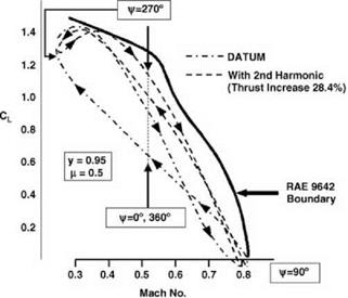
A calculation provided by Westland Helicopters illustrates the aerodynamic situation. The investigation consisted in comparing thrust performances of two rotors with and without second-harmonic control, of quite small amplitude – about 1.5° of blade incidence. Local lift conditions near the tip were monitored round the azimuth and related to the CL-M boundary of the blade section. The results shown in Figure 6.38 indicate that second-harmonic control gave an advantage of at least 0.2 in lift coefficient in the middle Mach number region appropriate to the disc fore and aft sectors.
|
Figure 6.38 Use of second-harmonic control: calculated example |
 This translated into a 28.4% increase in thrust available for the same retreating-blade boundary. A further advantage was that the rotor with second-harmonic control required a 22% smaller blade area than the data rotor, which, whether exploited as a reduction say from six blades to five or as a weight saving at equal blade numbers, would represent a considerable benefit in terms of component size and mission effectiveness.
A special drag problem relates to the design of the rear fuselage upsweep for a helicopter with rear loading doors, where the width across the back of the fuselage needs to be more or less constant from bottom to top.
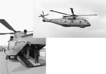
Figure 6.33 shows the difference in rear fuselage shape for a Merlin prototype in flight and a development (RAF) with a rear loading ramp door. In the 1960s, experience on fixed-wing
|
Figure 6.33 Shapes of Merlin fuselage both standard and that fitted with a rear loading ramp |
aircraft [13] revealed that where a rear fuselage was particularly bluff, drag was difficult to predict and could be considerably greater than would have been expected on a basis of classical bluff-body flow separation. Light was thrown on this problem in the 1970s by T. Morel [14,15]. Studying the drag of hatchback automobiles he found that the flow over a slanted base could take either of two forms: (1) the classical bluff-body flow consisting of cross-stream eddies or
(2) a flow characterized by streamwise vortices. Subsequently the problem was put into a helicopter context by Seddon [16], using wind tunnel model tests of which the results are summarized in Figures 6.34-6.37.
|
|
|
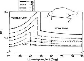
Figure 6.35 Variation of drag with upsweep angle at constant incidence |
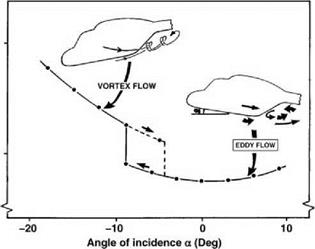
The combination of upsweep angle of the rear fuselage and incidence of the helicopter to the air stream determines the type of flow obtained. At positive incidence eddy flow persists. As incidence is decreased (nose going down as in forward flight) a critical angle is reached at which the flow changes suddenly to the vortex type and the drag jumps to a much higher level (Figure 6.34), which is maintained for further incidence decrease. If incidence is now increased, the reverse change takes place, though at a less negative incidence than before. The high drag corresponds to a high level of suction on the inclined surface, which is characteristic of the vortex flow. The suction force also has a downward lift component which is additionally detrimental to the helicopter. The type of flow is similar to that found on aerodynamically slender wings (as for example on the supersonic Concorde aircraft) but there the results are favourable because the lift component is upwards and the drag component is small except at high angle of attack.
|
|
|
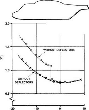
Figure 6.37 Vortex flow development prevented by deflectors |
The effect of changing upsweep angle is shown in Figure 6.35. Here each curve is for a constant fuselage incidence. With upsweep angles near 90°, eddy flow exists as would be expected. At a point in the mid-angle range of upsweep, depending on incidence, the flow change occurs, accompanied by the drag increase. As the upsweep angle is further reduced the drag falls progressively but there is a significant range of angle over which the drag is higher than in eddy flow.
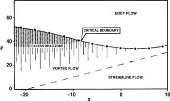
As an aid to design, the situation can be presented in the form of an a-f diagram, f being here the upsweep angle. The full line in Figure 6.36 is the locus of the drag jump when incidence is decreasing. If required, a locus can be drawn alongside to represent the situation with incidence increasing. Below the critical boundary is the zone of excess drag. From such a diagram, a designer can decide what range of upsweep angles is to be avoided for the aircraft. Of associated interest is the broken line shown: this marks an estimated boundary between vortex flow and streamlined flow, that is when no separation occurs at the upsweep. General considerations of aerodynamic streamlining suggest that the flow will remain attached if the upswept surface is inclined at not more than 20° to the direction of flight, in other words when f — a < 20°.
The final diagram, Figure 6.37, shows that if vortex flow occurs naturally, it can be prevented by an application of short, closely spaced deflectors on the fuselage side immediately ahead of the upswept face. The action is one of preventing the vortex from building up by cutting it off at multiple points along the edge.
Parasite drag – the drag of the many parts of a helicopter, such as the fuselage, rotor head, landing gear, tail rotor and tail surfaces, which make no direct contribution to main rotor lift – becomes a dominant factor in aircraft performance at the upper end of the forward speed range. Clearly the incentive to reduce parasite drag grows as emphasis is placed on speed achievement or on fuel economy. Equally clearly, since the contributing items all have individual functions of a practical nature, their design tends to be governed by practical considerations rather than by aerodynamic desiderata. Recommendations for streamlining, taken on their own, tend to have a somewhat hollow ring. What the research aerodynamicist can and must do, however, is provide an adequate background of reliable information which allows a designer to calculate and understand the items of parasite drag as they relate to their particular requirement and so review their options.
Such a background has been accumulated through the years and much of what is required can be obtained from review papers, of which an excellent example is that of Keys and Wiesner [10]. These authors have provided, by means of experimental data presented non-dimensionally, values of fuselage shape parameters that serve as targets for good aerodynamic design. These include such items as corner radii of the fuselage nose section, fuselage cross-section shape, afterbody taper and fuselage camber. Guidelines are given for calculating the drag of engine nacelles and protuberances such as aerials, lights and handholds. Particular attention is paid to the trends of landing-gear drag for wheels or skids, exposed or faired. Obviously the best solution for reducing the drag of landing gear is full retraction, which, however, adds significantly to aircraft weight. Keys and Wiesner have put this problem into perspective by means of a specimen calculation, which for a given mission estimates the minimum flight speed above which retraction shows a net benefit. The longer the mission, the lower the breakeven speed.
The largest single item in parasite drag is normally the contribution from the rotor head, known also briefly as hub drag. This relates to the driving mechanism between rotor shaft and
 |
blades, illustrated in Figure 6.29, and includes as drag components the hub itself, the shanks linking hub to blades, the hinge and feathering mechanisms and the control rods. Conventionally all these components are non-streamlined parts creating large regions of separated flow and giving a total drag greater than that of the basic fuselage, despite their much smaller dimensions. The drag of an articulated head may amount to 40% or 50% of total parasite drag, that of a hingeless head to about 30%. The application of aerodynamic fairings is possible to a degree, the more so with hingeless than with articulated heads, but is limited by the relative motions required between parts.
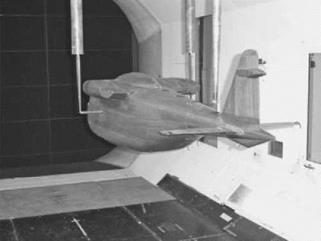
Sheehy [11] conducted a review of drag data on rotor heads from US sources and showed that projected frontal area was the determining factor for unfaired heads. Additionally, allowance had to be made for the effects of local dynamic pressure and head-fuselage interference, both of which factors increased the drag. Fairings needed to be aerodynamically sealed, especially at the head-fuselage junction. The effect of head rotation on drag was negligible for unfaired heads and variable for faired heads. The determination of helicopter hub drag is a very complex process and is often achieved by wind tunnel testing. A typical installation is shown in Figure 6.30.
Picking up the lines of Sheehy’s review, a systematic series of wind tunnel model tests was made at Bristol University [12], in which a simulated rotor head was built up in stages. The drag results are summarized in Figure 6.31.
An expression for rotor head drag D emerges in the form:
with the following definitions.
q0 is the free stream dynamic pressure X/2pV’^. q is the local dynamic pressure at the hub position, measured in absence of the rotor head. In a general case, the local supervelocity and hence q can be calculated from a knowledge of the fuselage shape.
CD is the effective drag coefficient of the bluff shapes making up the head. This may be assumed to be the same as for a circular cylinder at the same mean Reynolds number. For the
![]()
|
Figure 6.30
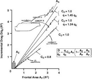 |
results of Figure 6.31 it is seen that a value CD = 1.0 fits the experimental data well, apart from an analytically interesting butunreal case of the hub without shanks, where the higher Reynolds number of the large-diameter unit is reflected in a lower CD value. In default of more precise information it is suggested that the value CD = 1.0 should be used for general estimation purposes. One might expect the larger Reynolds number of a full-scale head to give a lower drag coefficient, but the suggestion rests to a degree on Sheehy’s comment that small-scale model tests tend to undervalue the full-scale drag, probably because of difficulties of accurately modelling the head details.
|
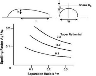
Figure 6.32 Chart for estimating spoiling factor AS |
AP is the projected frontal area of the head, as used by Sheehy. AZ represents a relieving factor on the drag, illustrated in Figure 6.31 and resulting from the fact that the head is partly immersed in the fuselage boundary layer. In magnitude AZ turns out to be equal to the projected area contained in a single thickness of the boundary layer as estimated in absence of the head. The last quantity AS represents in equivalent area terms the flow spoiling effect of the head on the canopy. This is a function jointly of the separation distance of the blade shanks above the canopy (the smaller the separation, the greater the spoiling) and the taper ratio of the canopy afterbody (the sharper the taper, the greater the spoiling). The ratio AS/AP may be estimated from the chart given in Figure 6.32 constructed by interpolation from the results for different canopies tested.
In light of the evidence quoted, the situation on rotor head drag may be summed up in the following points:
• The high drag of unfaired rotor heads is explained in terms of exposed frontal area and interference effects and can be calculated approximately for a given case.
• Hingeless systems have significantly lower rotor head drag than articulated systems.
• The scope for aerodynamic fairings is limited by the mechanical nature of the systems but some fairings are practical, more especially with hingeless rotors, and can give useful drag reductions.
• The development of head design concepts having smaller exposed frontal areas carries considerable aerodynamic benefit.
 |
 |
The following data are used:
This produces the graph in Figure 6.28.
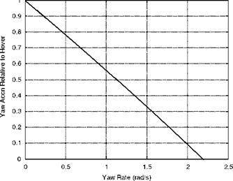
The figure shows the yaw acceleration attainable with the rotor on the point of stall. The yaw acceleration is normalized with the value in steady hover – that is, no yaw rate. Notice that, as the yaw rate increases, the thrust potential reduces as the precessional effects emerge by limiting the collective pitch which can be achieved before part of the tail rotor enters stall – in this case a yaw rate of 2.2rad/s.
|
Figure 6.28 Yaw acceleration limit due to precession caused by yaw rate |
The phenomenon of gyroscopic precession is somewhat esoteric but it plays an important influence on tail rotor performance. To a first look, gyroscopic precession seems to disobey what is a natural understanding of the effect of moments on a body. The simple toy of a spinning top placed on a small tower seems to defy gravity. Instead of falling to the ground, it moves around a vertical axis only slowly leaning further and further, spiralling towards the ground plane on which the tower is standing. Figure 6.20 shows the top in question.
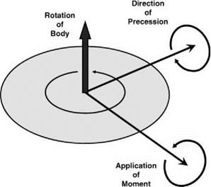
Using the right-hand rule, the top rotation and angular momentum are shown aligned with the spindle. The direction of the gravitational moment on the top is shown pointing to the right. The basic law is that the moment gives the rate of change of angular momentum. Hence the effect of gravity (and the reaction from the tower) will cause the angular momentum of the top to move in the same direction and thus the top rotates around the vertical axis in the precessional direction as shown. In Figure 6.21, the essential requirement is shown.
With reference to the rotational direction of the spinning body, the precessional rotation follows the applied moment by 90°.
The apparent avoidance of gravity is not a miracle, it just requires the moments and rotational directions to be expressed by vectors and then the standard laws apply – which they must!
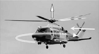
The tail rotor will encounter precession principally in the spot turn manoeuvre. This is where the helicopter is in hover and, by applying an increase/decrease in tail rotor thrust, spins about an axis along the main rotor shaft. This is illustrated in Figure 6.22, where the aircraft is rotating nose-left.
The tail rotor disc will have to rotate about a vertical axis, even though it is rotating about the rotor shaft. In order for this to happen, the rotor must have an appropriate precessional moment applied to it – as described in Figure 6.23.
|
Figure 6.21 Precessional moment |
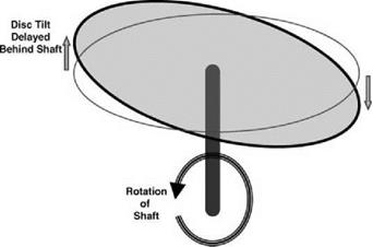
This moment cannot be achieved by any other means than aerodynamic, since the blades are not rigidly attached to the rotor shaft. With a fixed collective pitch and no cyclic pitch provision, the only way a moment can be generated is by blade flapping. It is important to note that lift variation is dependent on blade flapping velocity and not flapping displacement. Bearing this in mind, Figure 6.24 shows a rotor, where there is a disc tilt caused by a flapping displacement. The flapping velocities can be seen to be 90° out of phase with the flapping displacement. We therefore have two phase angle changes to consider, which results in the rotation of a rotor about an axis in the plane of rotation as shown in Figure 6.25. The rotor disc flaps in a direction lagging behind the shaft movement – the two 90° phase angles sum to give a total phase change of 180°.
|
|
|

 |
It can be shown that the rotation of a tail rotor about a vertical axis will generate a disc tilt of magnitude:
![]() Disc tilt
Disc tilt
(6.10)
 |
|
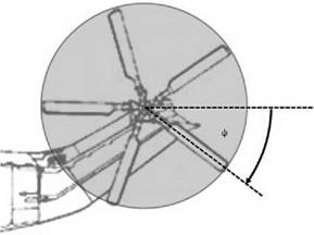
With the azimuth definition shown in Figure 6.26, a spot turn manoeuvre will cause a disc tilt which can be seen to be of a variety.
Figure 6.24 Relationship between flapping amplitude and flapping velocity
|
If we also consider the provision of pitch-flap coupling via a S3 hinge, the incidence of a typical blade is:
= 00-b-b tan S3- 7ZD
 |
The values of VZ and VJ are to be assumed constant over the rotor disc. Hence the Vz term will represent the value at the centre of the rotor. The VJ value will be defined by actuator disc theory
in climb at the appropriate value of VZ. We define the flapping angle and velocity as:
![]() b = a0—a cos ф b’ = a sin ф
b = a0—a cos ф b’ = a sin ф
 |
|
from which we find from (6.11):
 |
||
from which we must have:
![]()
![]() VZD
VZD
a = 60—a0 tan d3—a1sec d3 • sin^—d3)———
Or
This will have an extreme value of:
a = 60—a0 tan d3 + a1 sec d3 — —Z—
Or
If the blade is not to experience stall – taking the blade tip, as it has the highest Mach number – the collective pitch will be limited by this condition giving the stall incidence, aS, that is:
= as + a0 tan 03— a sec 03 + (mZ + 1i) Now the rotor thrust will be given by:
 |
which becomes:
The normalized climb rate is given by:
_ F • ^BOOM
Fz = VTT
. (6.24)
_ ^BOOM
Ot Rt
Using momentum theory we obtain:
Ctt = 41i(mZ + li) (6.25)
For the limiting case where the extreme rotor blade tip is at the point of stall, we must have from (6.21) and (6.25):
CTT Max = 41i Max (Fz + Ai Max)
![]()
 |
CTT Max aS mZ Ai Max 16 F
= – ;——- – sec d3 •
sa 3 6 6 3g OT
These can be combined to give:
![]()
|
|
|||
|
||||
|
|
|||
![]()
|
|
|
|
|
|
|
|
|
|
|
|
|
|
|
|
|
|
|
|
 |
|
|
|
|
|
|
|
|
|
|
|
|
|
 |
|
|
|
![]()
|
|
 |
|
|
|
|
|
|
|
|
|
|
|
|
|
|
|
|
|
|
|
|
|
 |
|
|
|
|
|
|
|
|
|
|
|
|
|
|
|
|
|
 |
|
|
|
|
|
Hence, the yaw acceleration is given by the excess tail rotor thrust over the steady hover value. We can now examine the ratio of the excess tail rotor thrust at zero yaw rate and at a spot turn yaw rate giving the maximum yaw acceleration as:
 |
|
C Max _ TT Max TTH C H Tth Max Tth
K ■ Ctt Max 1 K ■ CttH Max 1
where:
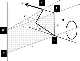
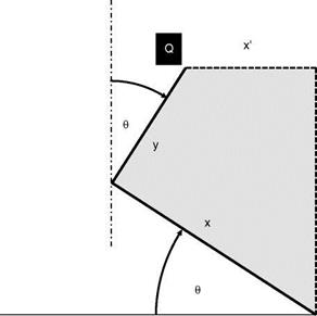
With reference to Figure 6.16, consider a point of a blade at Q. It is positioned on a blade section defined by the plane PP’Q and with a zero-pitch blade has the coordinates x (chordwise) and y
|
F
|
(thickness); however, the blade is rotated by an angle в and the position of Q can be defined by the coordinates x’ and y’.
Now Q will experience a centrifugal forcing term F in the direction shown in the figure. This will have a component, FX, in the direction normal to the radial line through P, the origin of the blade rotation. This will exert a moment about the axis OP in the direction of opposing the blade pitch rotation with a moment arm, y’. This is the propeller moment and is given by:
M = FX • y’ (6.1)
The forces F and FX are in a plane normal to the rotor shaft passing through the point Q. The transformation from (x, y) to (x’, y’) can be seen using Figure 6.17.
We therefore have the relations:
![]()
![]()
![]() x’ = x cos в—y sin в y’ = x sin в + y cos в
x’ = x cos в—y sin в y’ = x sin в + y cos в
To evaluate the force component, FX, Figure 6.18 shows the plane O’P’Q. Now the centrifugal force F is given by:
F = O2r’ dm
where dm is the elemental mass of the blade at point Q.
Resolving gives:
FX = F sin d
|
![]()
|
|
|
|
|
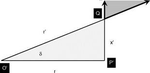
whence the force component is given by:
FX = O2r0 dm • sin d = O2 dm • r’sin d = O2 dm • x’
and the elemental propeller moment now becomes:
dM = FX • і
= O2 dm • X • і
= O2 dm(x cos в—y sin 0)(x sin в + y cos в)
= O2 dm [(x2—y2)sin в cos в + xy(cos2 в—sin2 в)]
|
O2 dm |
![]()
![]() , 2 sin2в . .
, 2 sin2в . .
(x2—y2) + (xy) cos 2в
|
x2—y2) sin 2в + xy (cos 2в) |
|
x2 dm |
Finally, by integrating over the blade:
![]() y2 dm
y2 dm
BLADE
BLADE
If the tail rotor aerofoil is symmetric, the product of inertia, /XY, vanishes, whence (6.7) simplifies to:
1 о
Mprop = 2O (/XX — Iyy)sin20 (6.8)
To this is added the aerodynamic pitching moment giving:
1 2
Mtotal = 2O (/xx — /yy)sin 2У + Maero (6.9)
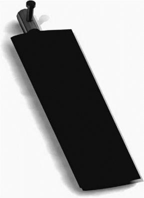
This pitching moment has to be reacted by the control system. For obvious reasons this has to be kept under limits of structural integrity and handling qualities – the pilot should not be expected to provide large forces on the pedals. The mechanism for adjusting the overall pitching moment is the bracketed term containing the difference of the two inertias. The moment can be increased by using /XX and decreased using /YY. Adjusting /XX is relatively easy since the blade layout is predominantly in the chordwise direction; however, /YY is not so easy as it can only be adjusted in the blade in the thickness direction, which is substantially lower because of the aerofoil section. To allow for this, the value of /YY is varied by means of an external mass added to the blade construction. It is usually mounted on the blade cuff as shown in Figure 6.19. These are termed preponderance weights.
|
|
|
|
|
|
|
|
|
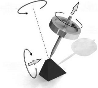
Figure 6.20 Precessing top