Category COMPUTATIONAL AEROACOUSTICS

It will be assumed that the function f(x), to be extrapolated, has a Fourier transform /(a). f(x) and /(a) are related by

TO

f (x) = J f (a) eiaxda. (11.9)

— TO

For convenience, let the absolute value and argument of f(a) be A and ф, respectively, i. e.,

A (a) = |/(a)| and ф(а) = arg[ f(a)]

so that Eq. (11.9) may be rewritten as

f (x)=/ A(a)‘iax+t’n’d

A simple interpretation of Eq. (11.10) is that f(x) is made up of a superposition of simple waves with wave number a and amplitude A (a). The primary goal here is to develop an extrapolation scheme that is highly accurate over the low wave number range, say, – к < a Ax < к. For this purpose, it will be sufficient to consider waves with unit amplitude over the desired band of wave numbers. The simple wave with wave number a to be considered is

f (x) = ei[ax+<p(a)]

11.1 Extrapolation and Numerical Instability

Extrapolation and interpolation are often used in large-scale computation. Here, extrapolation and interpolation on a regular mesh will be considered first. Interpo­lation on an irregular mesh will be discussed in Chapter 13. Most textbooks treat interpolation in great depth, but few discuss extrapolation. Some books state “extrap­olation should only be used with great caution.” The warning is proper and real. It is a well-known fact in scientific computing that extrapolation often leads to numerical instability.

The most popular method for interpolation and extrapolation is the method of Lagrange polynomials. Suppose an N-point computation stencil with a mesh spacing Ax is used to extrapolate the values of a function f(x) to the point x0 + n Ax (n < 1) (see Figure 11.1). Without the loss of generality, x0 will be taken as the first stencil point. The Lagrange polynomials formed by the N mesh points are

(N. N—1 (x – x,)

lk)(x) = , k = 0,1, 2,(N – 1) (11.1)

j=0 (xk – xj) j=k

It is easy to verify that

j = 0,1, 2,…, (N – 1)

j = k

The extrapolated value of f at n Ax, according to the Lagrange polynomials method, is given by

N-1

f(x0 + nAx) f (xj)lf ) x + nAx), (11.2)

j=0

where f(x), j = 0,1,…, (N – 1), are the given values of f at the mesh points.

Despite the popularity of the Lagrange polynomials method, there is no known way to assess the errors quantitatively. Standard estimates given in textbooks are obtained by expanding the left and right sides of Eq. (11.2) by the Taylor series for
small Ax. This way yields an error of the order of 9N f/dxN |x (Ax)N if N mesh points are used for extrapolation. This error estimate is, however, not at all useful.

To provide an example of numerical instability arising from the use of the Lagrange polynomials extrapolation and to show that such an instability can be avoided by using an improved method, the problem of acoustic wave propagation and reflection in a long one-dimensional tube with a closed end will now be considered. The problem is shown schematically in Figure 11.2. Dimensionless variables with Ax as the length scale, a0 (sound speed) as the velocity scale, Ax/a0 as the time scale, p0 (ambient gas density) as the density scale, p0a2 as the pressure scale will be used. It will be assumed that the end wall of the tube is not at a mesh point, but at a distance n (n < 1) from the last mesh point at I = 0. The governing equations are the linearized momentum and energy equations.

d u d p

+ = 0 dt dx

d p d u

+ = 0. dt dx

The wall boundary condition is

u = 0 at x = n.

Suppose the problem is solved on a mesh as shown in Figure 11.2. To reduce dispersion error, the standard 7-point stencil central difference scheme (sixth order)

is selected to approximate the x derivatives. The semidiscretized forms of Eqs. (11.3) and (11.4) are

d + £ ajPi+j = 0 (11.6)

j=-3

d-d – + £ ajUe+j = 0. (11.7)

j=-3

Near the wall where a 7-point central difference scheme cannot fit, backward difference stencils are to be used. Since the wall is not at a mesh point, the value of и at the wall may be obtained by extrapolation using the values of и at the nearest 7 mesh points. Suppose Lagrange polynomials extrapolation is used. The wall boundary condition (11.5) becomes

6

J2u-kl(k} = 0. (11.8)

k=0

The ghost point method will be used to enforce this boundary condition. For this purpose, a ghost value of pressure is introduced at the ghost point I = 1. The ghost value is chosen so that Eq. (11.8) is satisfied at every time level of the computation.

Tam and Kurbatskii (2000) have solved this discretized problem analytically. Their solution reveals that for n > 0.42, this discrete system is numerically unstable. The system supports one boundary instability mode with time dependence e—imt where ю = mr + imi is the complex angular frequency. If юі is positive, the mode is an unstable mode. This instability can also be determined computationally by solving Eqs. (11.6) to (11.8) using a time marching scheme such as the fourth-order Runge – Kutta scheme. Figure 11.3 shows the computed value of рг at I = -3 as a function of time. By measuring the oscillation period and amplitude, the angular frequency юг and growth rate юі can be found. As shown in Figure 11.4, the numerically determined values of юг and юі are in good agreement with the analytical results.

The observed numerical instability of the acoustic wave reflection problem is due entirely to the use of Lagrange polynomials extrapolation formula. It will be shown later that, by using an improved extrapolation scheme, there is no numerical instability.

In this third example, the scattering of acoustic modes by a circumferential splices is considered. The computational model is shown in Figure 10.14. For this test case, the width of the circumferential splices is taken to be 2Ax. For this size splice, there are only 2 mesh points on the splice surface (Ax = 0.008).

Consider the function F(x) defined by

where xc is the location of the center of the splice and W is its width. By means of the F(x) function, the wall boundary condition for a liner with a single circumferential splice may be written as

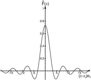Figure 10.21. The F (x) function. Wac = 2.5.

Now, the Fourier transform of F(x) is

Following the concept of the wave number truncated method, the high wave number components of Eq. (10.58) are to be removed at this stage. The truncated F(a) function is

e-laxc ( aw

F (a) = sin [H (a + ac) — H (a — ac)]. (10.59)

na 2

The inverse of F(a) is easily found to be 1

I7 (x) = [Si((x — xc + 0.5W )ac) — Si((x — xc — 0.5W )ac)]. (10.60)

n

A graph of I7(x) is given in Figure 10.21. The modified boundary condition to replace Eq. (10.57) is

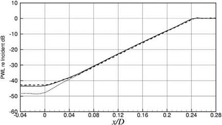
Figure 10.22 shows the results of four computations for duct mode scattering by a circumferential splice of width 0.02 located between x = 0.11 and 0.13. The incident duct mode and the liner impedance are the same as in Section 10.6.1. The first three computations use boundary condition (10.57). The mesh size used in the first computation is Ax = 0.002. There is spurious acoustic scattering at the upstream end of the splice. The axial distribution of the acoustic PWL is the uppermost broken curve in Figure 10.22. The second and third computation use a mesh size of Ax = 0.0005 and 0.00025, respectively. It is clear from this figure that the spurious scattering diminishes with the use of a finer mesh. The fourth computation uses modified boundary condition (10.61) and a very coarse mesh of Ax = 0.008. This is 32 times the size of the finest mesh used. For this computation, there are only 2 mesh

Figure 10.22. Duct mode scattering by a circumferential splice of width 0.02. Inci­dent wave mode and liner impedance are the same as Figure 10.16. Compar­ison of transmitted PWL: computed by

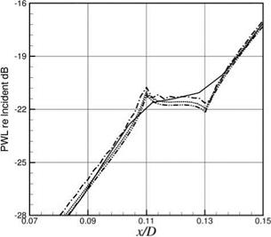boundary condition (10.61)—— Ax =

0.008; the following computed by bound­ary condition (10.57): Ax = 0.002,

…………… Ax = 0.0005, — • • — Ax =

0.00025.

points on the splice. The computed axial distribution of PWL is shown as the full line in Figure 10.22. For the transmitted PWL, which is one of the important quantities of the duct mode transmission computation, it is clear that the fourth computation using a mesh size 32 times larger gives almost identical results similar to those of the finest mesh. This example further illustrates the advantage of the wave number truncation method.

EXERCISES 10.1. Consider a single-frequency sound field of frequency О adjacent to an acous­tically treated panel or acoustic liner as shown in Figure 10.3. In other words, all the flow variables have the form p(x, y, z, t) = Re{p(x, y, z)e_iQt} when the solution has reached a time periodic state. Let the impedance of the liner be Z = R – iX. Verify that the following time-domain impedance boundary condition

d-P = R d-Vn _ xOvn

dt dt 11

yields the correct frequency-domain impedance boundary conditionp = Zvn.

Show by examining the dispersion relation of the acoustic field that boundary condition (A) is stable only when X < 0.

10.2. An acoustic wave train of frequency О = 1.6 kHz is sent down the normal incidence impedance tube shown in Figure 10.9. In dimensionless form, the incident wave is given by

Pincident = ^incident = cos[^(x _ t)] = Re _Ч •

The dimensionless resistance and reactance of the treatment panel are R = 0.18, X=-0.598, respectively. Compute the reflected wave train using boundary condition (A) of Problem 10.1. For this purpose, set up an incoming wave boundary condition on the left side of the computational domain. On the right side, use the ghost point
method to enforce the time-domain impedance boundary condition. Run your code long enough to attain a time periodic state before collecting numerical results.

Compare the pressure envelop inside the tube with that of the exact solution. The exact solution is

Preflected = Re {AeiQ(X+t} } , Mreflected = – Re {AeiQ(X+t} } ,

where A = (Z – 1)/(Z + 1). Note: Inside the normal incidence impedance tube the incident and the reflected wave train form a standing wave pattern. The maximum pressure amplitude at every point inside the tube form the pressure envelop.

10.3

Repeat Exercise 10.1 but replace boundary condition (A) by the following

Verify that time-domain impedance boundary condition (B) also leads to the correct frequency-domain impedance boundary condition p = Z vn. Show that (B) is stable only when X > 0.

10.4 Repeat Exercise 10.2 but at a higher frequency of 3 kHz. At this frequency, the resistance and reactance of the treatment panel are R = 0.18, X = 0.678. Use time-domain impedance boundary condition (B) in your computation. Compare your computed pressure envelop with the exact solution.

This example involves acoustic mode scattering by two thin axial splices. The com­putational model is shown in Figure 10.13. The same computational grid (see Figure 10.15) as in the previous subsection is used. The azimuthal mesh size of the outer­most ring of the cylindrical mesh is equal to 0.0123. Here, the acoustic scattering by two thin hard wall splices with a width of 0.006 is studied. It is noted that the splice width is approximately half of that of the mesh spacing (see Figure 9.15). In other words, the splices are invisible to the discretized computation.

Consider the periodic function, О(ф), of period 2п, defined by

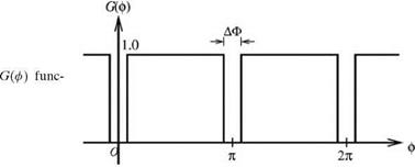°, -1АФ <ф<М п — Аф<ф<п + Аф

Ь(ф) =

1, otherwise

where АФ is the angle subtended by a splice. A graph of О(ф) is shown in Fig­ure 10.18. When applied to the surface of the duct, О(ф) = 1 where there is acoustic liner. It is equal to zero where there is hard wall splice. By means of the G-function, the wall boundary condition in the duct may be written as

Now, G^) is a period function; it may be expanded as a Fourier series. It is easy to find that

TO

G(ф) = ^ aj cos (]ф),
j=0

where

It is clear from Fourier expansion (10.52) that the G^) function contains compo­nents that are beyond the resolution of the 7-point stencil DRP scheme. To compute

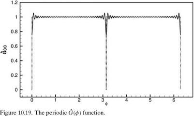acoustic wave propagation in the duct, these high wave number components essen­tially make the splice invisible to the computational mesh. A simple way to make the spliced liner compatible with the numerical scheme is to remove all Fourier components with azimuthal wavelengths shorter than the cutoff wavelength of the computational algorithm. Accordingly, all Fourier components with mode number m larger than mc, where the wavelength of mode mc is the same as or is closest to the smallest resolved wavelength of the computation scheme. For the cylindrical mesh used in the present computation, the azimuthal mesh size at the outermost ring is equal to 0.0123. For the 7-point stencil DRP scheme, acAx = 1.2, so that ac = 1.2/0.0123 = 97.6. Hence, by equating mc to the integer value closest to ac/2, it is found that mc = 49. Figure 10.19 shows the graph of the truncated Fourier series, G(ф) (Fourier components with m greater than 49 are removed), i. e.,

m

c

G(ф) = ^2 aj cos(]ф). (10.54)

m=0

The modified spliced liner boundary condition is to replace Є(ф) by G (ф) in Eq. (10.51), i. e.,

Figure 10.20 shows three computed PWL distributions along the length of the duct for the same incident duct mode as Section 10.6.1. In this computation, boundary condition (10.48) is used in the neighborhood of the liner hard wall junction at the two ends of the computational model. The dotted line in Figure 10.20 shows the numerical result when boundary condition (10.51) is used. There is no scattering in this case because the splices are invisible to the computational mesh. The full line is the computation using modified boundary condition (10.55). There is a large difference between these two curves. The difference is the energy of the scattered waves that are clearly quite substantial at the duct inlet. To check the accuracy of the wave number truncation method, a third computation using the quasi-two-dimension

azimuthal mode expansion method of Tam et al. (2008). This method expands the propagating acoustic waves in a large number of azimuthal modes. For the present computation, modes up to (mc + 40) are included. As a result of the large number of modes, the computation requires very large computer memory and long CPU time. The dashed curve of Figure 10.20 is the computed result using this method. It is evident that the result is very close to that of the wave number truncation method. This example offers a rigorous test of the effectiveness and accuracy of the wave number truncation method for computing the scattering of acoustic waves by narrow scatterers.

At the entrance or the exit of an inlet duct, there is a surface discontinuity at the junction of the liner and hard wall (see Figure 10.12 or Figure 10.14). These junctions invariably cause significant spurious scattering of a propagating duct mode. The scattering is an artifact of discrete computation. It can be reduced by using a finer size mesh or by implementing the wave number truncation method of Section 9.6.

The governing equations of motion of the gas inside an inlet duct are the lin­earized dimensionless Euler equations. In cylindrical coordinates, these equations are

where M = u/a0 is the flow Mach number.

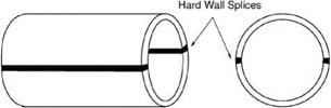Figure 10.13. Computational model of an inlet duct with two axial splices.

On the duct surface, the hard wall boundary condition is

1

‘ = 2’ V = °-

On the liner surface, the boundary condition is Eq. (10.19). At the left-hand junction of the computational model (Figure 10.12), the hard wall and liner boundary conditions can be combined to form a single boundary condition by means of the unit step function H(x). The combined boundary condition is

9 v d2v 9 p 9 p

RTT, – X-1v + X a? = H(x) { + Mi

Note: On the hard wall, x < 0, the H(x) function of boundary condition (10.47) is zero. This reduces the right side of the equation to zero. With the initial condition v = d v/д t = 0, the only solution is v = 0. In implementing the wave number truncation method, boundary condition (10.47) is replaced by

dv d2v 9 p d p

Rm – X-‘v+w=11 <x> і+Mі

where H(x), the truncated unit step function, is given by Eq. (9.67).

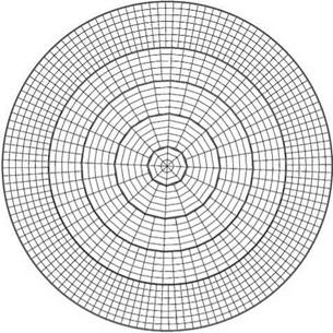
A cylindrical mesh, as shown in Figure 10.15, is used to compute the propaga­tion of acoustic modes upstream from the hard wall region on the right side of the

Figure 10.15. Cylindrical grid for duct acoustic mode computation. half the mesh lines are shown.

inlet model of Figure 10.12 to the left side. A uniform size mesh in the axial direc­tion is used. Now, consider an incident duct mode with azimuthal mode number m = 26 and radial mode number n = 1 and a dimensionless angular frequency ^ = 0.573. For such an acoustic mode, an axial mesh with Ax = 0.008 will allow the computation to have more than 8 mesh points per axial wavelength. This is the mesh used in all the computations of this section unless explicitly stated otherwise. In the computation, the 7-point stencil dispersion-relation-preserving (DRP) scheme is used to approximate the derivatives. The multimesh-size, multitime-step DRP scheme (see Chapter 12) is used to march the solution in time. The duct wall bound­ary conditions (liner impedance, Z = 2 + i, time factor exp(-i^t)) are enforced by the ghost point method. Recently, this method has been used successfully by Tam et al. (2008) in their spliced liner study. On the left and right end of the computa­tional domain, a perfectly matched layer (PML) is implemented. The PML absorbs all the outgoing waves. The incident acoustic mode, which enters the computational domain on the right side, is introduced into the computation by the split-variable method as discussed in Section 9.1.

Figure 10.16 shows the axial distribution of computed acoustic energy flux (PWL) associated with an incident duct mode with azimuthal mode number 26 and other parameters as stipulated above. PWL is the total energy flux of all the sound waves in the duct. It is defined as 2n 1/2

J j ((1 + M2)pu + M(p2 + u2)) тйтйф, 00

where () is the time average. PWL(dB) = 10 log (PWL/PWLincidentwave). This form of energy flux was derived by Morfey (1971). Of particular interest here are the computed results near the left junction between acoustic liner and hard wall. In this region, the effect of scattering of spurious acoustic waves is most severe and

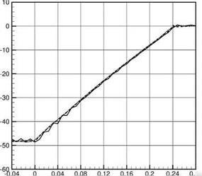
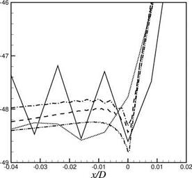Figure 10.16. Axial distribution of PWL. Incident wave has azimuthal mode number m = 26, radial mode num­ber n = 1, angular frequency Q = 0.573. Liner impedance Z = 2 + i

(time factor e-iQt).——— , Computed by

boundary condition (10.47), Ax = 0.008;

——- , computed by boundary condition

(10.47), Ax = 0.001; …… computed by

boundary condition (10.48), Ax = 0.008.

x/D

easily observable. The full line in this figure is the computed axial distribution of PWL using boundary condition (10.47) and axial mesh size 0.008. This curve exhibits strong spatial oscillations with a wavelength nearly equal to two axial mesh spacings. This is clear evidence of spurious scattering. The dotted line is the same computa­tion, but with a modified boundary condition (10.48). The computed distribution of PWL is smooth and free of spatial oscillations. This indicates that the wave number truncation method is indeed capable of removing spurious numerical scattering. To check the accuracy of the computed results by this method, a series of computations using boundary condition (10.47) is carried out with smaller and smaller axial mesh size Ax. Ax equals 1/4, 1/8, and 1/16 of the original mesh size used. The results near the left side liner-hard wall junction are shown in Figure 10.17 in an enlarged scale. As can be seen, as Ax is reduced, the computed result approaches that using boundary condition (10.48) but with a much larger Ax. The fact that there is good

Figure 10.17. Enlarged bottom left-hand corner of Figure 10.16. Computed by

boundary condition (10.47);——- , Ax =

0.008;——– , Ax = 0.002;———– , Ax =

0.001; — • • —, Ax = 0.0005; Computed

by boundary condition (10.48);…. Ax =

0.008.

agreement between results using much smaller Ax and boundary condition (10.47), and that using boundary condition (10.48) but much larger Ax, is evidence that the spatial oscillations of the full curve is of numerical origin. Further, it shows that the method of wave number truncation is effective and accurate. It also offers large savings in computer memory and CPU time.

Inside the inlet or the exhaust duct of a jet engine, the continuous reflections of acoustic waves by the walls lead to the formation of coherent propagating wave entities called duct modes or acoustic modes. These duct modes were first found by Tyler and Sofrin (1962) and have been the subject of numerous studies since. To suppress the duct modes, acoustic liners are commonly used. Because of installation and maintenance issues, a single large piece of liner is seldom used. A practical way is to install several smaller pieces of liners separated by hard wall splices. The presence of hard wall splices causes the scattering of the duct modes generated by the rotating fan blades of the engine. The scattered duct modes would, inevitably, include lower-order spinning azimuthal modes. The lower-order modes are not as heavily damped by the acoustic liner. This results in a higher level of radiated noise from the engine. This is extremely undesirable.

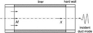
In this section, three numerical examples are presented to illustrate the effec­tiveness and accuracy of the time-domain impedance boundary condition and the wave number truncation method (see Section 9.6) for computing acoustic wave propagation and scattering in ducts with material discontinuities. These examples have practical relevance to jet engine duct acoustics. The inlet duct of a jet engine generally has a nearly circular geometry. The inside surface is covered by an acoustic liner. The liner occupies the space between two hard wall surfaces. One hard wall surface is the metallic surface surrounding the fan of the engine. The other hard wall surface is the lip of the engine inlet. Acoustic or duct modes are generated by the rotating fan of the engine. The duct modes propagate from the fan face upstream against the flow. They are radiated out from the inlet. A simplified model of the inlet duct is shown in Figure 10.12. This model has been used by numerous investigators for computing duct/acoustic mode propagation in jet engine ducts; e. g., Regan and Eaton (1999), McAlpine et al. (2003), Tester et al. (2006), and Tam et al. (2008). For a number of practical reasons, it is a standard practice to install hard wall splices

Figure 10.12. A computational model of the inlet duct of a jet engine.

to separate a liner into smaller pieces. Two types of splices are used. The more common type is the axial splice. An axial splice runs along the entire length of the liner. Figure 10.13 shows an inlet duct with two axial splices. Instead of axial splices, circumferential splices are often used. These splices form a ring around the inside surface of the duct. A duct with a circumferential splice is shown in Figure 10.14.

In the following examples, dimensionless variables are used. The scales of the various variables are: length scale D (diameter of the duct), velocity scale a0 (speed of sound), time scale D/a0, density scale p0 (mean flow density), pressure scale p0a2, and impedance scale p0a0.

To illustrate how well the time-domain impedance boundary condition works, con­sider an initial value problem associated with the normal-incidence impedance tube (see Figure 10.9). An impedance tube is designed to measure the impedance of an acoustic liner sample. Let the length of the impedance tube be 1.8 m. The speed of sound at room temperature is 340 m/s. To ensure that there are at least 7 mesh points per wavelength in the computation for sound frequency up to 4 kHz, the impedance tube is divided into 150 mesh spacings yielding Ax = 0.012 m. In this example Ax is used as the length scale; i. e., L = Ax. The impedance of the treatment panel is taken to be R = 0.18, X_x = -0.47567, and X1 = 2.09236 (a is nondimensionalized by a0/Ax). These are values corresponding to those of Figure 10.2. At time t = 0, a transient acoustic pulse is generated. This produces a broadband pressure field in the frequency domain. A part of the acoustic pulse propagates down the tube and impinges on the acoustic treatment panel on the right. This leads to a partially reflected pulse. It will be assumed that the disturbance is generated by the following initial conditions at t = 0:

u = 0, p = e_0 00444(x+83333)2 cos [0.444 (x + 83.333)]. (10.29)

Figure 10.9. A normal incidence impe­dance tube.

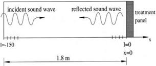This choice of initial conditions ensures that the center of the acoustic spectrum of the incident wave at the surface of the acoustic treatment panel has a frequency of 2 kHz and a spectrum half-width of 0.5 kHz The impedance tube problem has an exact solution, which may be derived as follows.

The governing equations for the acoustic field are the one-dimensional version of Eqs. (10.6) and (10.7). They are

The first term of Eq. (10.33) is the part of the pulse that propagates in the positive x direction. This is the sound pulse that impinges on the acoustically treated panel at x _ 0. For convenience, a subscript “inc” will be used to label the incident acoustic field, a subscript “ref” will be used to label the reflected field. Thus, the incident wave is

1

pmc _ umc _ 2e-000444(x-t+83’333)2 cos [0.444 (x – t + 83.333)]. (10.34)

Let

pref _ – uref _ Ф(x + t).

Eq. (10.35) is a general solution of Eq. (10.32). At the impedance surface, x _ 0, the Laplace transforms of the incident and reflected acoustic field variables are

On imposing the impedance boundary condition (10.1), one finds

(pmc + p ref ) = 7(umc + uref )• (10.38)

On using Eqs. (10.36) and (10.37), it is found that

7 — 1

Ф = 77+^1 P’mc^ (10.39)

The exact solution is obtained by taking the inverse transform of (10.39) and adjust the argument according to Eq. (10.35). This gives

(7 — 1)

g—56.265(®+0.444)2 + g—56.265(®—0.444)2

(7 + 1)L + –

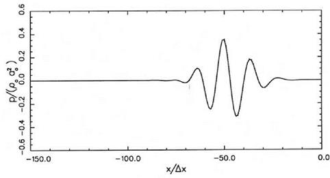
Figure 10.10 shows the computed pressure distribution at time t = 60.1. At this time, the left half of the initial pulse is about to exit the computational domain, whereas the right half of the pulse is about to impinge on the surface of the treatment panel. The dotted curve is the exact solution. Figure 10.11 shows the reflected pulse propagating away from the impedance boundary of the tube at t = 140.1. The amplitude of the reflected pulse is considerably smaller than that of the incident pulse. Part of the acoustic energy is dissipated off the impedance surface during the reflection process. The exact solution is represented by the dotted curve (the dotted curve is difficult to see because it is almost identical to the computed result). There is excellent agreement between numerical results and the exact solution. This is true for both the wave amplitude and phase. This example provides confidence in the use of time-domain impedance boundary condition.

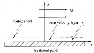
In jet engines, there is invariably a mean flow adjacent to the acoustic liners. Tradi­tionally, impedance boundary condition in the presence of a mean flow is formulated with the assumption of the existence of a very thin zero-velocity fluid layer at the sur­face of the acoustic liner (see Figure 10.6). At the interface of the zero-velocity fluid layer and the mean flow, the condition of continuity of particle displacement is used. In dimensionless variables the frequency-domain impedance boundary condition on liner surface S0(x, y, z) = 0, derived by Myers (1980), is

rnvnZ + (-іш + U-V) p = pn-(n-V )U,

where U is the mean flow velocity on the liner surface, n is the unit outward pointing normal of S0; that is, n = VS0/|VS0|. vn is the velocity normal to S0 with positive pointing into the liner. If the three-parameter model for Z is used, the time-domain impedance boundary condition is

For the special case for which S0 is a plane as shown in Figure 10.6, the frequency – domain impedance boundary condition, after simplification, may be written as

— іш + M—^ = – rnZvn. (10.13)

9 x

In an extensive numerical study of the normal modes of a duct with acoustic lin­ers, Tester (1973) found that boundary condition (10.13) led to an unstable solution. The unstable solution is of the Kelvin-Helmholtz-type instability arising from the vortex sheet interface between the mean flow and the zero-velocity fluid layer. In standard duct acoustics analysis using the frequency-domain approach, this instabil­ity is either not mentioned or totally bypassed and ignored. Now, it is easy to show that the use of boundary condition (10.13) always gives rise to an unstable solution.

The linearized momentum and energy equations governing the sound field superimposed on a uniform mean flow of Mach number M in the x direction (see Figure 10.6) are as follows:

where O = ю — Ma, к = (a2 + в2)1/2, and O = O/к. The branch cuts of the square root function (O2 -1)1/2 are the same as those stipulated in Figure 10.4 with O replacing о and к set equal to 1.

Substitution of solution (10.16) into the Fourier-Laplace transforms of boundary condition (10.13) yields the following dispersion relation:

Now, let the left side of Eq. (10.17) be denoted by f (O) as follows:

Figure 10.7 shows the map of the upper-half O plane in the f plane (shaded region) for X > 0. Since a can be positive or negative, there will always be values of a for which the point representing the right side of Eq. (10.17) lies in the shaded region of the f plane. Therefore, there will always be an unstable solution. If X is negative, a similar mapping procedure will show that there is always an unstable solution.

The existence of a Kelvin-Helmholtz-type instability renders the boundary value problem ill-posed for the time-domain solution. The instability is, however, non­physical. Its origin is in the postulate of a vortex sheet discontinuity right next to the impedance boundary. In reality, no such vortex sheet exists in the flow. For time-domain problems, the instability is weak. It can be effectively suppressed by the addition of artificial selective damping near and at the surface of the acoustic liner. With the weak instability suppressed, boundary condition (10.13) has yielded solutions that are in agreement with frequency-domain calculations.

Figure 10.7. Map of the upper-half a> plane in the f plane (X > 0): (a) a> plane, (b) f plane.

10.1 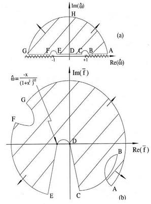Numerical Implementation

On incorporating the effect of convection (see Eq. (10.13)) the time-domain impedance boundary condition (10.4) or the Myers (1980) boundary condition

becomes

^+m ^ = я Ті – X v + X dt + dx dt -1 " + 1

The numerical implementation of this boundary condition will considered.

Let a large acoustically treated panel be lying on the x-z plane as shown in Figure 10.3. It will be assumed that there is a uniform flow adjacent to the panel. The governing equations of the acoustic field are the linearized Euler equations. In dimensionless form, these equations are

Now consider a computational domain as shown in Figure 10.8. y = 0 is the surface of the acoustically treated panel. Eqs. (10.20) to (10.24) apply to every grid point on the mesh. This includes the boundary points at y = 0 or m = 0, where m is the mesh index in the y direction. However, boundary condition (10.19) also applies to the boundary mesh point at y = 0 or m = 0. This means that there are more equations than unknowns. To resolve this problem of an overdetermined system, a row of ghost values of pressure, pe _1 k is introduced at m = -1, the ghost point. Here, subscripts I and к are the mesh indices in the x and z directions, respectively. Including the ghost values, the number of equations and unknowns are exactly equal. Since the ghost values are not governed by a time-dependent equation, it is necessary to combine boundary condition and equations of motion to reduce one of the equations effectively to a form without a time derivative. This form of the boundary condition is then used to determine the ghost values.

To facilitate the implementation of the time-domain impedance boundary con­dition (10.19), an auxiliary variable q(x, z, t), defined at y = 0 by

is introduced. q is only defined on the acoustic liner surface; i. e., y = 0. Note: vn = – v for the flow configuration of Figure 10.3. Boundary condition (10.19) may be rewritten, after eliminating дp/дt by Eq. (10.24), as follows:

^ = q _ m^. (10.27)

dy dx

Eq. (10.27) does not contain time derivative. It is in a suitable form for use to determine the ghost value pl -1k.

The discretized form of Eq. (10.27) using the backward difference stencil of Figure 10.8 is

where Ax and Ay are the mesh sizes. On solving for the ghost value, it is straightfor­ward to find

On choosing the ghost value by Eq. (10.28), the governing Eq. (10.27) or its progenitor Eq. (10.22) is automatically satisfied. To compute the entire sound field, the values of p, u, w, and p at every mesh point (l, m, k) are calculated by Eqs. (10.20), (10.21), (10.23), and (10.24). For velocity component v at all mesh points, except those on the acoustically treated panel surface, i. e., m = 0, the value is updated by means of Eq. (10.22). For mesh points at m = 0, vl,0,k are computed by Eq. (10.25). The auxiliary variable q is to be calculated by Eq. (10.26). In discretizing the spatial derivatives in y for mesh points in rows m = 0,1,2, the backward difference stencils shown in Figure 10.8 are to be used. Finally, artificial selective damping must be added to each time-dependent equation to suppress the weak instability of the impedance model.

The time-domain impedance boundary condition (10.4) may not be used unless it leads to a stable solution. To show that an acoustic problem with (10.4) as boundary condition is computationally stable, consider a plane acoustic liner adjacent to a sound field as shown in Figure 10.3. For simplicity, let the surface of the liner be the x-z plane. In terms of dimensionless variables with L (a typical length of the problem) as the length scale, a0 (the sound speed) as the velocity scale, L/a0 as

Figure 10.3. Sound field adjacent to an acoustically treated panel.

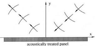the time scale, p0 (the gas density) as the density scale, p0a2 as the pressure scale, and p0a0 as the scale for impedance, the acoustic field equations (the linearized momentum and energy equations) are as follows:

£=-Vp (106)

f = – V-v. (1°.7)

Let f (а, в, o) be the Fourier-Laplace transform of a function f(x, z, t). The functions f and f are related by

TOTO

f(a, fi, w) = —3 j j j f (x, z, t)e-l(ax+ez-mttdtdxdz (10.8a)

-TO 0 TO

f ) = f(a-e^ax*-^da de (108b)

— to Г

By applying Fourier-Laplace transforms to Eqs. (10.6) and (10.7), it is easy to find that the solution that satisfies the radiation and boundedness condition as

y ^ TO is

(10.9)

where k = (а 2+ в2)1/2, and v is the velocity component in the y direction (note that v = – vn). The branch cuts of the function (o2 – k2)1/2 are taken to be 0 < arg(o2 –

k2)1/2 <

n, the left (right) equality is to be used if o is real and positive (negative). The branch cut configuration in the o plane is shown in Figure 10.4.

The Fourier-Laplace transform of Eq. (10.4) is

– op = [-oR0 + i(X— 1 + a>2X1 )]vn. (10.10)

Substitution of Eq. (10.9) into Eq. (10.10) results in the dispersion relation as follows:

2

1

(o2 – k2) 2

Figure 10.4. Branch cut configuration for (ю2 – к2)1/2. Argument of (ю2 – к2)1/2 =

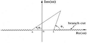
2 (Ф1 + Ф2)

That is, F(w) is the left side of Eq. (10.11). By tracing over the contour ABCDEFGH in the upper-half ю plane, it is easy to establish that the upper-half ю plane is mapped into the shaded region in the F plane as shown in Figure 10.5. The mapped region does not include the negative imaginary axis. Now X-1, on the right side of Eq. (10.11), is negative. This means that no value of ю in the upper-half ю plane would satisfy dispersion relation (10.11). Thus, the solutions of the initial value problem

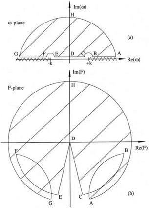Figure 10.5. Map of the upper-half ю plane in the F plane. (a) ю plane, (b) F plane.

Figure 10.6. Schematic diagram show­ing a postulated zero-velocity fluid layer adjacent to an acoustically treated panel in the presence of a mean flow.

can only have ы with a negative imaginary part. These solutions are numerically stable.

A simple model for the broadband impedance boundary condition is to take the resistance R to be a constant and the reactance X to be given by Eq. (10.2). That is,

where R0 > 0, X-1 < 0, X1 > 0.

For this model, the time-domain impedance boundary condition may be written as follows:

It is straightforward to show, by assuming time dependence of the form e~imt for all variables, that Eq. (10.4) is equivalent to the frequency-domain impedance boundary condition with impedance given by Eq. (10.3).

For a single-frequency sound field of frequency Q (Q > 0), this three-parameter model may still be used. Let Z0 = R0 – iX0 be the impedance of the acoustic liner at frequency Q, then the following choice of X-1 and X1 will transform the broadband model to a single-frequency model.