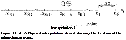
Our heavyweight helicopter equal in the world does not have
In Rostov started production of the most load-lifting rotary-wing car The Russian holding «Helicopt[...]

Everything about aircrafts and helicopters. News and events in aviation worldwide. Civil, transportation, military helicopters and airplanes.

Everything about aircrafts and helicopters. News and events in aviation worldwide. Civil, transportation, military helicopters and airplanes.

Everything about aircrafts and helicopters. News and events in aviation worldwide. Civil, transportation, military helicopters and airplanes.

Everything about aircrafts and helicopters. News and events in aviation worldwide. Civil, transportation, military helicopters and airplanes.


As discussed before, artificial selective damping is incorporated into the DRP computational algorithm for two purposes. First, it is used to provide background damping to eliminate short spurious waves to prevent them from propagating across the computation domain. Generally speaking, small-amplitude short spurious waves are just low-level pollutants of the numerical solution, but if these waves are allowed to impinge on an internal or external boundary of the computational domain, they could lead to the reflection of large-amplitude long waves. These spurious long waves are sometimes not distinguishable from the physical solution and are, therefore, extremely undesirable. The second reason to add artificial selective damping is to stabilize the numerical solution at a discontinuity. The damping prevents the buildup of spurious short waves, which are generated by the discontinuity, and this promotes stability.
In the present problem, the forcing functions are discontinuous at the blade tip. Thus, in addition to the general background damping with an inverse mesh Reynolds number 0.05, extra damping is added around the blade tip region. The mesh-size-change interface and the external boundary of the computation domain are also a form of discontinuity. Extra damping is added around these boundaries as well. To impose extra damping, a distribution of inverse mesh Reynolds number in the form of a Gaussian function with a half-width of four mesh spacings normal to the boundary is used. The maximum of the Gaussian is on the discontinuity with an assigned value of 0.05. At the tip of the blade, where the forcing function is discontinuous, more damping is required. A maximum value of 0.75 is used instead.
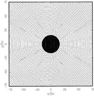
The half-width of the forcing function in Eqs. (12.30) and (12.31) is 0.2. To resolve this width, a minimum of 10 mesh points is necessary. In other words, the maximum mesh size in the source region is 0.02. This high resolution is not needed as one moves away into the acoustic field. The multi-size-mesh multi-time-step DRP algorithm is used for computation. This allows one to use coarser and coarser mesh starting from the source region radially outward. Figure 12.11 shows the computation domain. The domain is divided into three regions. The mesh size as well as the time step increases by a factor of 2 each time one crosses into an outer region.
12.4.1.2 Numerical Boundary Conditions
Two types of numerical boundary conditions are needed. Along the outer boundary of the computation domain, radiation boundary conditions are required. Along the axis of the cylindrical coordinates, i. e., r = 0, a special set of axis boundary conditions is needed. Here, the radiation boundary conditions are used as follows:
![]()
![]() (12.35)
(12.35)
where R = (r2 + x2)1/2.
As r ^ 0, Eq. (12.34) has a numerical singularity and cannot be used as it is. The situation is similar to that discussed in Section 9.4. By adopting the numerical
treatment of Section 9.4, the solution is extended to the negative r part of the x — r plane as follows:
й(—r, x) = (—1)mU(r, x) v(—r, x) = (—1)m—1 v(r, x) w (—r, x) = (—1)m—1tw (r, x)
p(—r, x) = (—1)mp(r, x) (12.36)
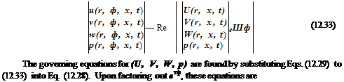
Formula (12.36) allows one to extend the computed solution into the lower half of the x — r plane as indicated in Figure 12.12. In this way, computation stencils for
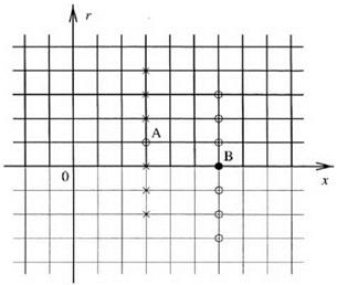
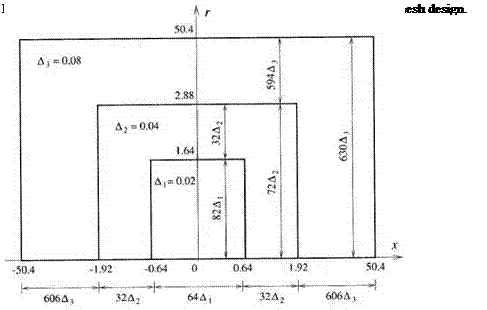
Figure 12.12. Extension of the computational domain, the upper part of the x — r plane, to the nonphysical lower half plane.
points near the axis (but not on the axis such as point A) may be extended into the negative r half-plane as shown. For the points on the axis, such as point B, they will not be calculated by the time marching DRP scheme. They are to be found, after the values at all the other points have been updated to a new time level, by symmetric interpolation. A 7-point interpolation stencil for point B is shown in Figure 12.12.
To illustrate the implementation and the effectiveness of multi-size-mesh multitime-step computing, two problems from the Third CAA Workshop on Benchmark Problems are considered here. The first is a two-dimensional rotor noise problem. The second is an automobile door cavity tone problem.
12.4.1 First Example: The Sound Field of an Open Rotor
For this problem, it is convenient to use nondimensional variables with respect to the following scales:
length scale = b(length of blade) velocity scale = a0 (ambient sound speed) time scale = b/a0
density scale = p0 (ambient gas density) pressure scale = p0 a0
body force scale (per unit volume) = p0a200/b
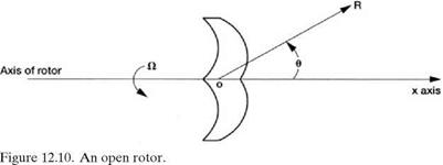
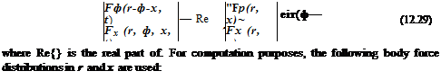
A rotor (see Figure 12.10) exerts a rotating force on the fluid. As a model problem, the rotor is replaced by a distribution of rotating body force. The governing equations are the linearized Euler equations. In cylindrical coordinates (r, ф, x), they
![]()
|
|
 |
|
 |
|
|
|
|
|
 |
|
 |
|
 |
|
|
|
For an open rotor solution, it is only necessary to find the outgoing wave solution of Eq. (12.34) in the r – x plane.
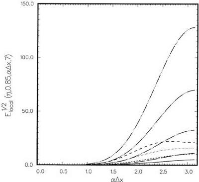
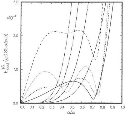
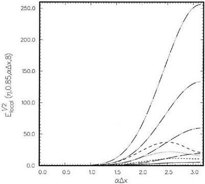
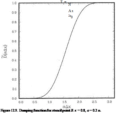
Now, the benchmark problem is to calculate the directivity, D (в), of the radiated sound for a eight-blade rotor (m = 8) with N = 1 (Л8д = 9.64742). In a spherical polar coordinates system (R, в, ф), with the x-axis as the polar axis, the directivity is defined by
D(e) = lim R2p2 (R, в, ф, t),
where an overbar indicates a time average. The directivity D(e) at one-degree interval at two rotational speeds
(a) ^ = 0.85 (subsonic tip speed)
(b) ^ = 1.15 (supersonic tip speed)
are to be computed.
To ensure that the computed solution is accurate, one must make provisions to take into account two important characteristics of this problem. First, the noise source is discontinuous at the blade tip. This could be a source of short spurious numerical waves. Second, the blades are slender, that is, the loading is concentrated over a narrow width. Computationally, this requires a finer spatial resolution in the source region than in the acoustic radiation field.
In numerical computation, surfaces of discontinuity, such as mesh-size-change interfaces, are potential sources of spurious numerical waves. For this reason, it is necessary to add artificial selective damping in the buffer region of the interface. For points A and A’, the 7-point damping stencils discussed in Chapter 7 may be used. For points B or B’, C or C special damping stencils are needed.
Consider the x-momentum equation of the linearized Euler equations.
I + = °- (1216)
The discretized form of Eq. (12.16) at point C, including the artificial selective damping terms, is
where the damping stencil coefficients satisfy the symmetric condition d— = d, va is the artificial kinematic viscosity, and Ax is the mesh size at C.
Consider a single Fourier component of u, i. e., u = u.(t)elaiAx. Substitution into Eq. (12.17) yields
(—^ +••• =———– —2DC (a Ax) u, (12.18)
dtJc (Ax)2 V ‘
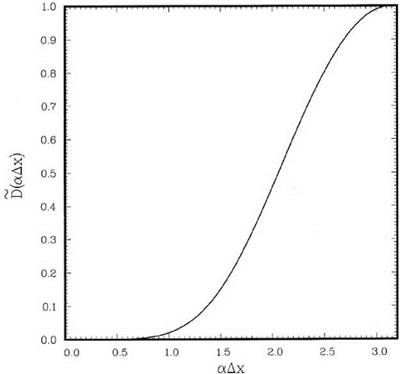
where the damping function DC(aAx) is given by
DC(aAx) = dC + 2 [dC cos(aAx) + dCcos(2a Ax) + dCcos(4a Ax)]. (12.19)
As in Chapter 7, it is required that there is no damping if u is a constant (or a Ax ^ 0). This leads to
3
dC + 2J2 dj = 0. (12.20)
j=1
The normalization condition is DC(n) = 1.0 or
dC + 2(-dC + dC + dC) = 1. (12.21)
In addition, it is intended to select the remaining parameters such that Eq. (12.19) is a good approximation to a Gaussian function of half-width a centered at a Ax = n. Specifically, the integral
|
Figure 12.8. Damping function for stencil point C. к = 0.7, a = 0.2 n. |
is to be minimized. Numerical experiments suggest that a good choice of к and a are
к = 0.7, a = 0.2n. (12.22)
This yields the following damping stencil coefficients:
dCC = 0.350576727483
dC = d-1 = -0.25
dC = d-2 = 0.0788677598279
dC = d-3 = -0.004156123569. (12.23)
The damping function corresponding to this stencil is shown in Figure 12.8.
On following these steps, the coefficients of the damping stencil for points B or B’ are found. In this case, numerical experiments suggest the choice of к = 0.8 and a = 0.2n. The damping stencil coefficients are as follows:
dB = 0.5
dB = dB1 = -0.294977493296 dB = dB2 = 0.052389707989
dB = dB3 = -0.007412214693. (12.24)
The damping function is shown in Figure 12.9.
 |
|
One is often required to compute flows with a thin boundary layer adjacent to a wall. To calculate such rapidly changing flows, it is desirable to use higher spatial resolution in regions with rapid changes. Thus, the finest mesh is installed right next to the wall. In such a mesh design, one may have a cascade of mesh sizes through several layers from the outermost coarse layer to the finest mesh layer right at the wall. Experience has shown that it is possible for waves corresponding to grid-to-grid oscillations to be trapped in one of the nested mesh layers very close to the wall. This provides an environment for the growth of grid-to-grid oscillations as they bounce from one side of the layer to the other side, gaining amplitude at each reflection. It is, therefore, a good practice to impose stronger artificial selective damping in the computation for the fine meshes near a wall. For an estimate of the magnitude of mesh Reynolds number that should be imposed, it is noted that the time, T, needed by the short waves to propagate from one side of the mesh layer to the other side, is equal to the distance traveled divided by the speed of propagation. Here, the group velocity of the spurious grid-to-grid oscillations is taken to be approximately equal to twice the speed of sound a0 (see Figure 2.4). Hence, one finds
where N is the number of mesh points across the width of the mesh layer, and Ax is the mesh size. The total damping in this time period is given by Eq. (7.15). Since D (n) = 1.0, the total damping factor is
![]() _ _VL ____ N_
_ _VL ____ N_
e (Ax)2 = e 2Ra,
|
|
where RA=va/(Ax)a0 is the mesh Reynolds number. It is suggested that this factor should be equal to 10-2 or less to avoid accumulation of spurious grid-to-grid oscillations. On setting this factor equal to 10-2, a criterion for the choice of the mesh Reynolds number is established, namely,
N
— > 9.2. (12.27)
ra
For example, if the nested mesh layer has 20 mesh points, i. e., N = 20, then Ra1 > 0.46, say 0.5, should be used. This value is much larger than the value recommended for general background damping, which is Ra1 > 0.05. (Note: away from the solid boundaries a smaller and smaller inverse mesh Reynolds number should be used.) Formula (12.27) also suggests that any uniform mesh layer in a multisize-mesh computation should not have fewer than 20 mesh points. This is to avoid the necessity of using excessively large artificial damping.
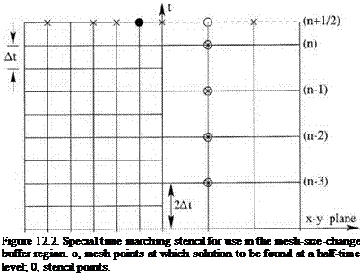
The time marching step, ft, is constrained by the numerical stability or accuracy requirements of a computation scheme. In general, the stability or accuracy requirements link ft directly to the mesh size fx. Thus, in a region with large mesh size, a larger ft may be used. When more than one mesh size is used, the optimum strategy is to use the largest time step permissible in each region. It follows, if the mesh size changes by a factor of 2 in adjacent domains, the time step should also change by the same ratio. Figure 12.2 shows the time levels of the computation in the mesh – size-change buffer region. In the fine mesh region on the left, the time step is ft. In the coarse mesh region on the right, the time step is 2ft. Effectively, the fine mesh region is computed twice as often as the coarse mesh region.
![]()
 Suppose the solution is known at time level n (see Figure 12.2), the solution in the fine mesh region may be advanced by a time step At to time level (n + 1 /2) in the usual way. Once this is completed, the next step is to advance the solution to time level (n + 1) in both the fine and coarse mesh regions. It is straightforward to carry out this step in the coarse mesh region by using the solution on time levels n, (n – 1), (n – 2), and (n – 3). However, for points in the buffer region on the fine mesh side, the stencils extend into the coarse mesh region. There is no information at the (n + 1/2) time level at these points on the coarse mesh side. To provide the needed information of the solution, it is necessary to compute the solution at the time level (n + 1 /2) for the first two rows or columns of the mesh point on the coarse mesh side based on the solution at time levels n, (n – 1), (n – 2), and (n – 3). To advance the solution by a half time step as shown in Figure 12.2, the following four-level scheme may be used:
where К = du/dt is given by the governing equation, and (l, m) are the spatial indices.
|
(e-iaAt -1) 3 Ul, m (2At )Y^ b*e2ijaAt |
To find the stencil coefficients b* of Eq. (12.9), one may consider u to be made up of a Fourier spectrum of simple harmonic components of the form e-iat, where a is the angular frequency. The effect of time marching algorithm (12.9) on each Fourier component of frequency a may be analyzed by substituting ufm = ulm (t) = Ae-lan(2At) into Eq. (12.9). It is easy to find
Since d(u m/dt)=iaul m, the factor, on the right side of Eq. (12.10), multiplying U m, must be equal to – ia, where a is the angular frequency of the time marching finite difference scheme. Thus, one finds that
![]()
![]() i(e-iaAt -1)
i(e-iaAt -1)
3
2 b*e2i1aAt
1=0 1
There are four coefficients, namely, b*0, b*, b2, and b. Here, the condition that a ~ a be accurate to order (At)[15] is imposed. On expanding Eq. (12.11) by the Taylor series, it is straightforward to find that the four coefficients are related by the following three conditions:
|
Figure 12.7. The dependence of the seven roots of юAt on a) At. |
There is no loss of generality regarding b0 as the remaining free parameter. The value of b0 is chosen so that ю is a good approximation of ю over the frequency band – X < юAt < X. This is done by minimizing the integral as follows:
A
E(bo) = j {a[Re(«At) — юAt]2 + (1 — a)[Im(«At)]2} d(o^At), (12.15)
-A
where a is the weight parameter. The condition for minimization is dE/db0 = 0.
A numerical study of the real and imaginary parts of («At — rnAt) for different choices of X and a has been carried out. Based on the results of this study, the values X = 0.5 and a = 0.42 are recommended for use. For this choice of parameters, the optimized coefficients are as follows:
b0 = 0.773100253426 b = —0.485967426944 b2 = 0.277634093611 b3 = —0.064766920092.
For a given «At, Eq. (12.11) yields seven roots of юAt. As in the original DRP scheme, only one of the roots yields the physical solution. All the other roots are spurious and should be damped if the scheme is to be stable. Figure 12.7 shows
the dependence of the roots on «At. The scheme is stable if «At < 0.88. If «At is restricted to less than or equal to 0.19, then the damping rate, Im(«At), is less than 0.78 x 10⁻⁵, which is quite small. The accuracy of this scheme when restricted to this range is comparable to that of the standard DRP scheme.
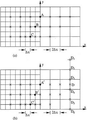
If a factor-of-2 increase in the mesh size between adjacent blocks is used, then every other mesh line in the fine mesh block continues into the coarse mesh block as shown in Figure 12.1. The remaining set of mesh lines terminates at the mesh-size-change interface. To compute the x derivative for points on the coarse grid, including points on the interface such as point A, the 7-point central difference DRP scheme may be used even though part of the stencil is extended into the fine mesh region. For mesh points on the fine grid, again the 7-point central difference DRP scheme may be used except for the first three columns (or rows) of mesh points right next to the coarse grid. For points on the continuing mesh lines such as points B and C in Figure 12.1, special central difference stencils, as indicated, are to be used. These stencils may be written in the following form:
To find the stencil coefficients aBj and aCC (j = -3 to 3), the optimization procedure of Chapter 2 may be followed. Now, first consider the stencil for point B. As in Section 11.2, it will be assumed that f(x) has a Fourier transform f(a) with absolute value A (a) and argument ф(а); i. e.,
A(a) = | f(a)|, ф(а) = arg[ f(a)|.
The Fourier transform may be written as
![]() f (x) = / A(a*"*-*d
f (x) = / A(a*"*-*d
In other words, f(x) is made up of a superposition of simple waves, fa(x), of the following form:
fa(x) = еТ“+ф(а)], (12.4)
weighted by A (a). Now the accuracy of finite difference approximation (12.1) of each simple wave component of f(x) is examined. Upon substituting fa (x) into Eq. (12.1), the finite difference approximation becomes
a fa(x) ~ a fa(x),
where
2
a = — aB sin (a Ax) + aB sin (3a Ax) + aB sin (5aAx)] (12.5)
is the wave number of the finite difference stencil. In deriving (12.5), the antisymmetric condition, a – j = – aB, has been invoked.
On following the steps of Chapter 2, the condition that Eq. (12.1) or Eq. (12.5) be accurate to order (Ax)4 is imposed. By means of Taylor series expansion, this condition yields the following restrictions on the stencil coefficients:
2(aB + 3aB + 5aB) = 1
aB + 33aB + 53 aB = 0 (12.6)
The coefficients will now be chosen so that the error of using a Ax to approximate a Ax over the band of wave number | a Ax| < к, E, is minimum subjected to conditions (12.6). For this purpose, the error is defined as к
![]()
![]() J [aAx – aAx]d (a Ax) 0
J [aAx – aAx]d (a Ax) 0
The condition for a minimum is given by (after eliminating aB and a3B by Eq.
An extensive numerical study of the effects of the choice of к on a(a) and da /da has been carried out. Based on the numerical results, it is deemed that a good choice
|
Figure 12.3. Dependence of a Ax on a Ax for stencil B. к = 0.85. |
of the values of к is 0.85. For this choice, the values of the stencil coefficients are
aB = 0.0
aB = aB1 = 0.595328177715 aB = aB2 = -0.037247422191 a3B = aB 3 = 0.003282817772.
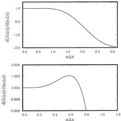
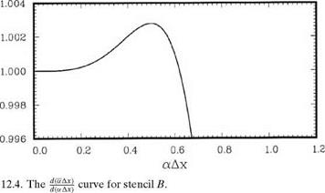
Figures 12.3 and 12.4 show the corresponding a(a) and dal da curves. The resolution and dispersion characteristics of the stencil lie in between those of the central difference DRP scheme on the two sides of the interface.
On proceeding as for stencil B, the stencil coefficients for stencil C may be found. For stencil C, it is recommended that the value к = 1.0 be used. The stencil coefficients are
aC = 0.0
aC = aCB1 = 0.726325187522 aC = aC2 = -0.120619908868 aC = aC3 = 0.003728657553.
Figures 12.5 and 12.6 show the corresponding a(a) and da/da curves for this stencil. Again, the resolution and dispersion characteristics lie in between those of the central difference DRP scheme on the two sides of the interface.
![]()
|
|
 |
|
Figure 12.6. The doff) curve for stencil C. |
For mesh points lying on the terminating mesh lines such as points A’, B’, and C of Figure 12.1, the same stencils as for A, B, and C may be used, However, the stencils extend into points in the coarse mesh region where the solution is not computed. To obtain the values of the solution at these points, such as point D, it is recommended that interpolation be used. The interpolation stencil, a symmetric stencil is preferred, makes use of the values of the adjacent 6 mesh points, D1 to D6, as shown in Figure 12.1. In actual computation, the interpolation step is executed only after the solution on the coarse mesh region has been advanced by a time step. The interpolated values allow the solution on the fine mesh side to continue advancing in time.
As an example on the use of extrapolation and interpolation in large-scale computing, the problem of scattering of plane acoustic waves by a cylinder in two dimensions is considered. Let the diameter of the cylinder be D. The governing equations are
![]()
 |
|
|
|
n = 0.75…………….. , к = 0.85;———– , к = 0.9; — • —, к = 0.95;————- , к
![]() к = 1.05;————- , к = 1.1;——– , Lagrange polynomials interpolation.
к = 1.05;————- , к = 1.1;——– , Lagrange polynomials interpolation.
 |
П = 0.75…………….. , к = 0.85;———– , к = 0.9;———- , к = 0.95;———— , к = 1.0;——– ,
к = 1.05;————- , к = 1.1;——– , Lagrange polynomials interpolation.
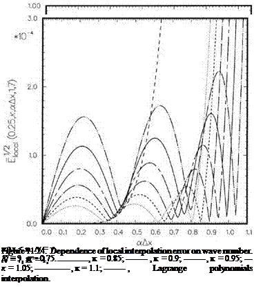 |
П = 0.25……………. , к = 0.85;——— , к = 0.9;———– , к = 0.95;———— , к = 1.0;
к = 1.05;————- , к = 1.1;———- , Lagrange polynomials interpolation.
the linearized Euler equations. In dimensionless form, they may be written as (with respect to length scale D, velocity scale a0 (speed of sound), time scale Dl a0, density scale p0, and pressure scale p0 a02).
![]()
d U d E d F
dt + 3^*" dy
where
|
p |
u |
v |
|||
|
U= |
1 і______ |
, E = |
P 0 u _ |
, F = |
0 P v |
On the surface of the cylinder, the boundary condition is V n = 0, where n is the unit normal to the surface. It can be shown easily that an equivalent form of the boundary condition is
¥ = 0- (11.35)
d n
Eq. (11.34) maybe discretized on a Cartesian mesh using the dispersion-relationpreserving scheme. The scattered sound field may be found by time marching the numerical solution to a time periodic state. However, because the cylinder has a curved surface, a special boundary treatment is needed to enforce boundary condition (11.35). For this purpose, the ghost point method has been extended to treat
Figure 11.26. Cartesian boundary treatment of curved wall surfaces.
arbitrarily curved wall boundaries (see Kurbatskii and Tam, 1997). As an illustration of the boundary treatment, consider the curved boundary shown in Figure 11.26. First, the boundary curve is approximated by line segments joining the intersection points of the computation mesh and the wall boundary. For instance, the curved surface between points A and B in Figure 11.26 is replaced by a straight-line segment. G2 is a ghost point. A ghost value of pressure is assigned to G2 to enforce boundary condition (11.35). The enforcement point is at E; G2E is perpendicular to AB. Since dp/дx and dp/дy are not known, except on the mesh points, their values at A and B are found by extrapolation from the points at (Г, 2′, 3′, 4′, 5′, 6′, 7′) and (1, 2, 3, 4, 5,6,7), respectively. The corresponding values at E are then calculated by interpolation from those at A and B. Once дp/дх and дp/ду are found at E, Eq. (11.35) can be enforced readily.
To show the impact of the extrapolation scheme used on the computed results of the scattered waves, a computation domain of 320 x 320 with Ax = Ay = D/32 is used in the solution of the scattering problem. The wavelength of the incoming acoustic waves is equal to 8 Ax. The method of numerical treatment of incoming plane acoustic waves of Section 10.1 is followed in the computation. Because of the special boundary treatment needed to enforce the curved wall boundary conditions, the accuracy of the computed scattered wave is greatly influenced by the extrapolation formula used. Figure 11.27 shows the computed zero pressure contours of the scattered waves at the beginning of a cycle when the Lagrange polynomials extrapolation method is used in the computation. Shown in dotted lines are the zero pressure contours of the exact solution. It is obvious that there are significant differences between
|
Figure 11.27. Zero pressure contours of the scattered sound field at the beginning of a cycle. Lagrange polynomials are used for extrapolation.——- , numerical results;………….. , exact solution. |
the two sets of contours. It is not difficult to understand why there are such large discrepancies. Wave number analysis indicates that, at 8 mesh points per wavelength, the Lagrange polynomials extrapolation method would give rise to large errors. Such errors contaminate the entire computed scattered wave field.
Figure 11.28 is an identical computation using the optimized extrapolation scheme with an added constraint. Clearly, there is excellent agreement between the numerical results and the exact solution. This is, of course, not surprising since the optimized extrapolation as well as the time marching algorithm are designed to yield fairly accurate results for waves with wavelengths of eight mesh spacings or longer.
EXERCISES [13] [14]
Determine the matrix system by which optimized extrapolation coefficients, Sj, can be calculated. It is suggested that the averaged spacing between adjacent stencil points, A, be used as the length scale.
11.2. Consider two-dimensional interpolation using a rectangular stencil of N by M mesh points. To find the interpolated value at a point P with coordinates (x0, y0), one may first find the values of the function at the intersection of line AA’ (see Figure 11.29) and the mesh lines by interpolation in the y direction. The next
step is to interpolate along AA’ for the value of the function at P. The alternative is to interpolate in the x direction first. That is, the values of the function at the intersection points on the line BB’ with the mesh lines are found by interpolation first. Then the values are interpolated along BB’ to obtain the value of the function at P. Show that the interpolated value at P is the same independent of which direction the interpolation is performed first.

 |
Many aeroacoustics problems involve multiple length and time scales. This should not be difficult to understand. For, in addition to the intrinsic sizes and scales of the noise sources, the acoustic wavelength is an inherent length scale of the problem. In many instances, the length scale of the noise source differs greatly from the acoustic wavelength. This leads to a large disparity in length scales as in classical multiscales problems. For example, in supersonic jet noise, Mach wave radiation is generated by the instability waves of the jet flow. The instability waves are supported by the thin shear layer of the jet. In the region near the nozzle exit, the averaged shear layer thickness is about 0.1D, where D is the jet diameter. The acoustic wavelength, on the other hand, is two or more jet diameters long. Thus, there is an order of magnitude difference between those characteristic lengths. In sound scattering problems, the length scale of the surface geometry of the scatterers may be much smaller than the acoustic wavelength. This occurs very often in edge scattering and diffraction problems. A concrete example is the radiation of fan noise from a jet engine inlet. The acoustic wavelength could be much longer than the radius of the lip of the engine inlet. To obtain an accurate numerical solution of the inlet diffraction problem, a fine mesh is needed around the lip region. Oftentimes, an aeroacoustics problem becomes a multiscales problem because of the change in the physics governing the different parts of the computational domain. An example is the shedding of vortices at the edge of a resonator or a sharp edge of a solid body induced by high-intensity incident sound waves. Away from the solid surface, the fluid is nearly inviscid, but close to the wall, the viscosity effect dominates. The oscillatory motion of the incident sound waves induces a very thin Stokes layer on the solid surface. The Stokes layer rolls up at the corner of a solid surface to form vortices that shed periodically. To simulate the vortex shedding process, therefore, it is necessary to use very fine mesh close to the solid surface and around the corner to resolve the Stokes layer. But away from the solid surface, a coarse mesh with 7 mesh points per acoustic wavelength is all that is needed to capture the sound waves accurately using the 7-point stencil dispersion-relation-preserving (DRP) scheme.
Computationally, a very effective way to treat a multiscales problem is to use a multisize mesh. Figure 12.1 shows a typical multisize mesh. In this example, the mesh size changes by a factor of two across the mesh-size-change interface. A factor-of-2 change in the mesh size is not an absolute necessity. It is recommended because a
Figure 12.1. Special stencils for use in the mesh-size-change buffer regions. •, mesh points at which finite difference approximation of spatial derivative is to be found; x, stencil points; o, points used for interpolation.
 larger change may result in a very strong artificial discontinuity inside the computational domain. On the other hand, a smaller change may require several steps of changes to achieve the same total change in mesh size. This will give rise to a large number of mesh-size-change interfaces, which is not desirable.
The time step used in a computation is dictated very often by the choice of spatial mesh size. Recall that numerical instability requirements link At, the time step, to the mesh size Ax. If a single time step marching scheme such as the Runge- Kutta method is used, then At is dictated by the smallest size mesh of the entire computational domain. This results in an inefficient computation. The optimum situation is to use a At consistent with the local numerical stability requirement. In such an arrangement, most of the computation is concentrated in regions with fine meshes, as it should be. In the coarse mesh region, the solution is updated only occasionally with a much larger time step. This type of algorithm is referred to as “multi-size-mesh multi-time-step” schemes. If the mesh-size change is a factor of 2 across the mesh block interface, the time step should also change by a factor of 2 to maintain numerical stability. For multilevel time marching schemes such as the DRP scheme, the use of multiple time steps with a factor-of-2 change between adjacent mesh blocks is easy to arrange. Figure 12.2 shows such an arrangement in which the computed solution advanced in steps of At in the fine mesh region and in steps of 2 At in the coarse mesh region.
In carrying out a multi-size-mesh multi-time-step computation, the computation scheme to be used in each of the uniform mesh blocks is the same as if there is a single
size mesh throughout the entire computation domain. The exception is for a narrow buffer region at the block interface. In the buffer region, special stencils are to be used so that information on the solution can be transmitted through without significant degradation. Also, note that any surface of discontinuity, no matter whether it is a mesh-size-change interface or an internal or external boundary, is a likely source of short spurious numerical waves. To suppress the generation of spurious short waves, special artificial selective damping stencils should be incorporated in the computation scheme for mesh points adjacent to the block interface. The design of these special stencils is given in the next three sections.
In this section, a wave number analysis of interpolation error is performed. At the same time, an optimized interpolation procedure is formulated. Interpolation is generally a numerically stable operation incurring relatively little error. For this
|
Figure 11.9. Same as Figure 11.8, except the full wave number range is shown. |
|
|
|
|
reason, one can only expect a relatively small improvement by using an optimized scheme.
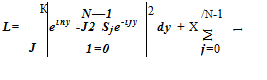
Consider an N-point interpolation stencil as shown in Figure 11.14. Let x0 be the first point of the stencil. The other stencil points are located at Xj = x0 – jAx (j = 1 to (N – 1)). Suppose the interpolation point is in the Kth interval of the stencil at a distance of nAx to the right of xK. The interpolation formula is
N-1
![]()
![]() Ev (xj )•
Ev (xj )•
j=0
 |
As before, the local interpolation error, £local, is defined as the square of the absolute value of the difference between the left and the right sides of Eq. (11.27) when the single Fourier component of Eq. (11.11) is substituted into the
Now, the interpolation coefficients Sj are chosen so that E is a minimum subjected to the condition that there is no error for zero wave number. The zero wave number condition may be written as
 |
N—1
 |
The Lagrangian function of this constrained minimization problem is
![]() Л Sj = 1
Л Sj = 1
j=0
The linear system Eq. (11.33) may be rewritten in a matrix form similar to Eq. (11.19). The matrix equation can be solved easily to provide the interpolation coefficients, Sj (j = 0,1, 2,…, (N—1)).
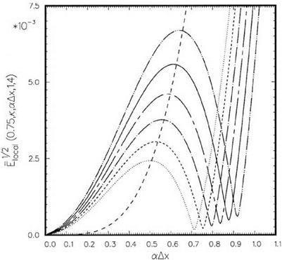
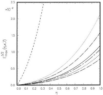
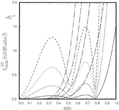
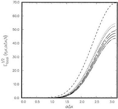
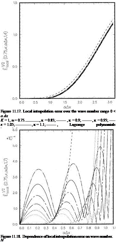
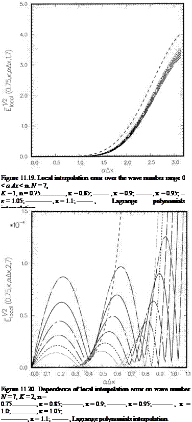
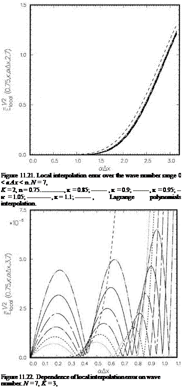
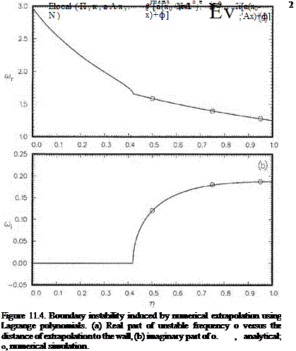
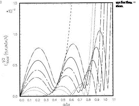
The local interpolation error Elocal as a function of wave number a Ax depends on a number of parameters. They are N (the stencil size), K (the interval number), n (the distance to the mesh point), and the free parameter к. Numerical results are now provided to offer an idea on the magnitude of the error and how it is influenced by the various parameters.
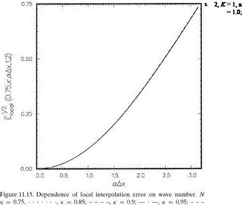 |
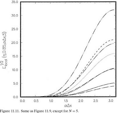
Consider first the effect of N, the size of the stencil. Figure 11.15 shows the distribution of Elocal in wave number space for n= 0.75 using only two interpolation points, N = 2. This is a very special case. The parameter к appears to have a negligible effect on the local error. In addition, the optimized scheme yields almost identical results as the Lagrange polynomials interpolation. The error is relatively large in the high wave number range, but relatively small at low wave numbers. The interpolation point will now be kept in the first interval of the stencil, i. e., K = 1, but the stencil size is allowed to increase. Figures 11.16 and 11.17 show the local error distributions as functions of wave number at various values of к with N = 4 or four interpolation points. On comparison with Figure 11.15, it is clear that, by increasing the size of the stencil, the error in the low wave number range drops rapidly. At the same time, the error in the high wave numbers increases. Figures 11.18 and 11.19 provide the results for an even larger stencil, N = 7. In this case, the low wave number error becomes negligible, but the error in the neighborhood of a Ax = n is much larger.
If the interpolation point lies in the interior of a large stencil, one intuitively expects much smaller error than when it is located at the first interval. Figures 11.20 and 11.21 show the numerical results for N = 7, n= 0.75, and K = 2. Figures 11.22 and 11.23 show the corresponding results for K = 3. These results completely confirm the intuitive expectation. Over the long wave range, a Ax < 0.9, there is hardly any error when the interpolation point lies in the center interval for large N
|
Figure 11.16. Dependence of local interpolation error on wave number. N = 4, K = 1, n = 0.75………….. , к = 0.85;——— , к = 0.9;——— , к = 0.95;———- , к = 1.0;——— , к = 1.05; ———— , к = 1.1;——– , Lagrange polynomials interpolation. |
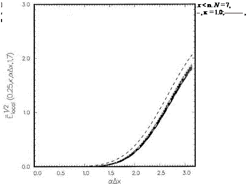
The effect of the distance of the interpolation point from the stencil point, namely, the magnitude of n will now be considered. Figures 11.24 and 11.25 give the local errors for n= 0.25. The values of the other parameters are the same as those of Figures 11.18 and 11.19. As readily seen, the two sets of figures are about the same. This indicates that n has a relatively small effect on the local error.
Finally, the effect of free parameter к is considered. After reviewing and comparing all the numerical results, it is found that a good overall choice for this parameter is 1.0. This value of к provides a large range of low wave numbers over which the interpolation error is small. At the same time, the error at high wave numbers is still numerically small. In most large-scale computations, the high wave number components will remain unresolved. They are the spurious numerical waves, which are suppressed by the inclusion of artificial selective damping or filtering. As a result, the amplitude of the high wave number components is expected to be small. Any amplification by the interpolation process would still be small. They should not be a concern except in unusual circumstances.
Figure 11.6 indicates that the extrapolation error for high wave numbers, particularly for a Ax near n, is very large. This means that, in a large-scale computation, the high wave number components can be greatly amplified by the extrapolation process. This observation suggests that it is this numerical error amplification mechanism that is responsible for the often encountered numerical instability associated with extrapolation. From this point of view, it would be desirable to keep the local error at a Ax = n and over the high wave number range smaller. This may be done by imposing an additional constraint on the optimization process. Suppose it is desired to fix the extrapolated error El1o/c2al of the function at a Ax = n to be a prescribed value, say, h(n). For this purpose, an additional condition,
|
is imposed. The first term of Eq. (11.21) is equal to the extrapolated value of the simple wave function fa(x) of Eq. (11.11) at aAx = n. Thus, for all intents and purposes, it is equal to the square root of the local error. By specifying the function h(n), one stipulates the maximum error allowed at aAx = n. Extensive numerical experiments have found that a good choice of h(n) is
h (n) = 1.0 + 19n. (11.22)
 |
|
Upon including Eq. (11.21) as an additional constraint, the Lagrangian function to be minimized is
The conditions for minimization are as follows:
dS = 0, j = 0, 1, 2,…, (N – 1), dX = 0, dX = 0. (11.24)
dSj dX dx
|
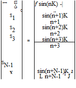
Eq. (11.24) may be recast into a matrix system as follows:
|
|
Г S ] |
~ sin^) ” n |
|
|
S1 |
n+1 |
|
|
S2 |
sin(n+2)к n+2 |
|
|
S3 |
= |
sin(n+3)к n+3 |
|
SN-1 X |
sin(n+N-1)к n+N-1 1 |
|
|
ft |
h(n) |
Eq. (11.25) may be solved easily by a standard matrix equation solver. Once S;-’s are found, the local error £local can be calculated. Figure 11.8 shows the variation of Еоы with wave numbers a Ax for к = 0.85, N = 7 at four values of n. For a Ax < 0.8 or 8 mesh points or more per wavelength, the maximum extrapolation error is less than
1.5 percent. Shown in this figure also are the local errors of the Lagrange polynomials extrapolation method. It is evident that for a Ax > 0.6, the error is huge. Figure 11.9 shows an identical plot but covers the entire range of wave numbers. Near a Ax = n, there is significant difference in the errors between the two extrapolation procedures. For instance, for n= 1.0, the Lagrange polynomials method has an error about six times larger than that of the optimized scheme. One would, therefore, expect that the improved optimized scheme is less likely to induce numerical instability.
Figures 11.10 to 11.13 provide similar information as Figures 11.8 and 11.9 at stencil sizes of 5 and 8. They illustrate the effect of using a smaller or larger extrapolation stencil. Generally speaking, the use of a larger stencil reduces the error in the low wave number range but increases the error at high wave numbers. This is a piece of useful information in deciding the proper stencil size to use.
As an example that the added constraint in the optimized extrapolation method does reduce numerical instability, the one-dimensional acoustic wave propagation and reflection problem of Figure 11.2 is again considered. Now the computation is
|
Figure 11.8. Local error as a function of wave number using the optimized extrapolation method with an added constraint. к = 0.85, N = 7. |
П optimized extrapolation Lagrange polynomials extrapolation
0.25—————- ————————————-
0.50 ——— ————————————-
0.75 ………… ………………………………………………
1.00 ————— —————————————- repeated using the optimized extrapolation scheme to find the value of u at the wall, x = n,; i. e.,
6
£>_ jSj (n) = 0. (11.26)
j=0
It can be shown analytically and demonstrated computationally (see Tam and Kurbatskii, 2000) that there is no boundary instability. In other words, the optimized scheme with the additional constraint has effectively eliminated the boundary instability mode created by numerical extrapolation using the Lagrange polynomials method.
Now, instead of Lagrange polynomials extrapolation formula (11.2), a more general formula,
(n-1)
f (X0 + nAx) = J2 Sjf (Xj), Xj = X0 – jAx, (11.12)
j=0
will be used, where Sj (j = 0, 1, 2,…, N-1)) are the stencil coefficients. Sj is unknown at this stage and Sj is equal to ljn) (x0 + n Ax) for the Lagrange polynomial
 |
|
extrapolation method. Now, the local extrapolation error for wave number aAx, Elocal(n, к, a Ax, N), is defined as the square of the absolute value of the difference between the left and right side of Eq. (11.12) when a single Fourier component of Eq. (11.11) is substituted into the formula as follows:
Note that Elocal(n, к, – a Ax, N) = Elocal(n, к, aAx, N).
The integrated error over the band of wave numbers from aAx = 0 to aAx = к
One expects the extrapolation error to be zero if the function is a constant or a = 0. From Eq. (11.13), this condition gives
fN-1
![]() J2Si – ^ = °-
J2Si – ^ = °-
j=0
Now, Sj, the coefficients of extrapolation formula (11.12), is to be chosen so that E is a minimum subjected to constraint (11.15). This constrained optimization problem can easily be solved by the method of the Lagrange multiplier. The Lagrangian function may be defined as follows:
 (11.16)
The coefficients Sj and the Lagrange parameter X are found by solving the linear system as follows:
![Подпись: sin4K sin[(N-1)K ] 1 “I 4 N-1 2 sin3K sin[(N-2)K ] 1 3 N-2 2 sin2K sin[(N-3)K ] 1 2 N-3 2 sin К sin[(N-4)K ] N-4 1 2 sin 2K ' ' 2 sin К К 1 2 ■ ■ 1 1 1 0](/img/3131/image958_0.gif) |
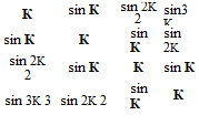 |
![Подпись: sin[(N-1)K] sin[(N-2)K ] N-1 N-2 1 1 1](/img/3131/image960_0.gif) |
Now, the integrals of Eq. (11.17) can be readily evaluated. The algebraic system of Eqs. (11.17) and (11.18) leads to the following linear matrix equation:
 (11.19)
In Eq. (11.19), к is a free parameter. This parameter is to be selected so as to offer the best overall results. Once Sjs are found, the local error Elocal may be
computed according to Eq. (11.13). Figure 11.5 shows the dependence of E^ on wave number aAx in the case n = 0.75 and N = 7 for several values of к. This figure is typical of other values of n and N. Plotted in this figure is also the local error of the Lagrange polynomials extrapolation. It is readily seen that the Lagrange polynomials extrapolation is very accurate for low wave numbers, but the error becomes large for a Ax > 0.6 or wavelengths shorter than 10.5 Ax. Many finite difference schemes used in large-scale computations and simulations can resolve waves longer than eight mesh spacings or a Ax < 0.85. Therefore, it would be incompatible to use the Lagrange polynomials extrapolation with these schemes. On the other hand, the local error of the optimized extrapolation is larger at very low wave numbers. The error up to a Ax = 0.85 is quite comparable to those of the high-order computational schemes. Figure 11.6 shows the distribution of local error over the full range of wave numbers, i. e., 0 < a Ax < n. Note that at aAx = n, the local error of the Lagrange polynomials method is exceedingly large.
To examine the variation of extrapolation error on n, let
This is the maximum error incurred in the extrapolation process if the function involved has a Fourier spectrum confined to the range aAx < 0.85. Figure 11.7 shows the dependence of Emax on n for the case N = 7. For к = 0.85, is less than
![]()
|
10- 2 for n up to 1.0. A similar investigation for N = 5,6, and 8 shows that Emax remains low if к is taken to be 0.85. Based on this numerical study, it is recommended that the parameter к be assigned the value 0.85 when used in connection with large-scale high-order finite difference computation.