Our heavyweight helicopter equal in the world does not have
In Rostov started production of the most load-lifting rotary-wing car The Russian holding «Helicopt[...]

Everything about aircrafts and helicopters. News and events in aviation worldwide. Civil, transportation, military helicopters and airplanes.

Everything about aircrafts and helicopters. News and events in aviation worldwide. Civil, transportation, military helicopters and airplanes.

Everything about aircrafts and helicopters. News and events in aviation worldwide. Civil, transportation, military helicopters and airplanes.

Everything about aircrafts and helicopters. News and events in aviation worldwide. Civil, transportation, military helicopters and airplanes.


An interpolation stencil may be regular or irregular depending on the configuration of the stencil relative to the coordinate system used for the computation. Generally speaking, interpolation error is small compared with extrapolation error. Figure
13.6 shows a 16-point irregular interpolation stencil. For reference purposes, the coordinates of the interpolation points of this stencil are as follows:
(-0.70,1.72) (0.34,1.58) (1.24, 1.14) (-1.62, 0.72) (-0.38, 0.79) (0.64, 0.60) (-1.02, 0.08) (0.18, -0.20) (1.58, 0.06) (-1.24, -0.56) (-0.38, -0.92) (0.80.-0.78) (-1.56, -1.40) (-0.26, -1.68) (0.66, -1.52) (1.64, -1.16)
The points to be interpolated are as follows:
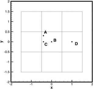
A (-0.40, 0.30)
B (0.00, 0.00)
C (-0.40, 0.00)
D (1.00,0.00)
Figure 13.7 shows a 16-point regular stencil in the form of a square. Interpolation error analysis for the 4 points A, B, C, and D shown in both Figures 13.6 and 13.7 have been carried out. The finding is that the errors for points A, B, and C are very similar. For this reason, only the interpolation errors of A and D will be discussed. It is useful to consider point A as typical of all the points located around the center of the stencil and point D as typical of all the points located close to the boundary of the stencil.
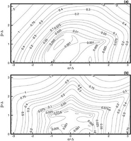
Figure 13.8 shows the local error, £local, contours in the аА – в A plane. In calculating £local, к has been set equal to 1.2. It has been found through numerical experimentation that к = 1.2 is a reasonably good value to use. As readily seen in Figure 13.8, unlike extrapolation, there is no large error even for high wave numbers.
|
|
|
In most aeroacoustics applications, the range of wave numbers that is of interest is -1.0 < a A, в A < 1.0. In order to show error maps with more clarity, only the low wave number portion of the а A – в A plane is shown in the discussions to be followed.
The imposition of order constraints has a significant impact on the local error distribution in the wave number space. Generally speaking, imposing high-order constraints is beneficial in reducing the error in the low wave number region. On the other hand, it tends to cause an increase in error in the high wave number region.
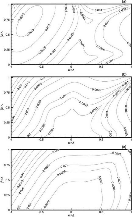
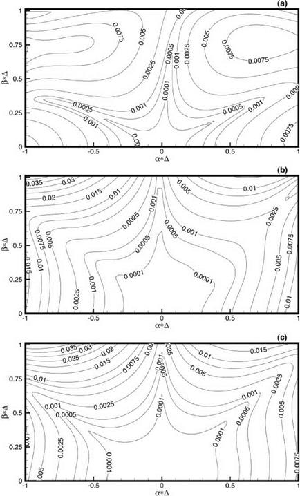
Figures 13.9a-13.9c show the error contour distributions in the а A – в A plane for interpolation to point A using the irregular stencil of Figure 13.6. Figure 13.9a is obtained with the imposition of a second-order constraint. Figures 13.9b and 13.9c are the results with the imposition of a third – and fourth-order constraint, respectively. It is clear from these figures that the best result or least error in the region -0.5 < aA, в A < 0.5 is realized by enforcing the highest-order constraint. On the other hand, if one is interested in keeping the error small over a larger region in wave number space, then the low-order constraint becomes attractive. For point A only the second-order constraint interpolation has an error less than 1 percent over the wave number region of -1.0 < aA, в A < < 1.0. Figures 13.10a-13.10c are for interpolation to point D of the irregular stencil. Again, the error contours of these figures point to the benefit of minimizing interpolation error over the low wave number range by using the maximum order constraints. The error is less than 0.25 percent for |aA |, ^A | < 0.55 (wave length longer than 12.5 mesh points). Again, for the larger wave number range, say -1.0 < aA, в A < 1.0, the second – order constraint has an interpolation error less than 1 percent. Thus, the choice of order constraints depends on the range of wave numbers one wishes to have the error below a specified level. For general usage, the imposition of a medium-order constraint (say second or third order for a 16-point irregular stencil) may be a good compromise.
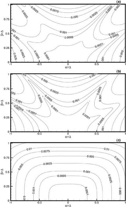
Figure 13.11 shows contours of local interpolation error, £local, at A using the 16- point regular stencil of Figure 13.7. Figures 13.11a-13.11c are subjected to second-, third-, and fourth-order constraints, respectively. Because of regularity of the stencil points, Xj = xk and yj = yk occur repeatedly, there are only four independent values of Xj and yj (j = 1,2,…, 16). This immediately leads to degeneracy in the fourth-order constraints. To show this is, indeed, the case, recall that the interpolation coefficients are to be found by solving Eq. (13.35) BX = d. Here, N is 16. Including the last row of submatrix A, the last 15 rows of matrix B are as follows:
|
1 |
1 |
1 •• |
1 |
0 ………….. |
……….. 0 |
||||
|
X1 |
– X0 |
X2 |
– X0 |
X3 |
– X0 •• |
‘ XN |
– X0 |
0 ………….. |
……….. 0 |
|
У1 |
– У0 |
y2 |
– У0 |
У3 |
– У0 •• |
‘ УN |
– У0 |
0 ………….. |
……….. 0 |
|
(X1 ■ |
– X0)2 |
(X2 |
– X0)2 |
(X3 ■ |
– X0)2 " |
‘ (XN |
1 * О |
0 ………….. |
……….. 0 |
|
(У1 ■ |
– У0 )4 |
(y2 |
– У0 )4 |
(У3 ■ |
– У0)4 •• |
■ CVn |
о •• i |
0 ………….. |
……….. 0 |
|
|
|
|
|
|
If there is no degeneracy, these fifteen row vectors must be linearly independent. But this is not the case as shown below.
Consider the following five of the fifteen row vectors:
|
1 |
1 |
1 |
1 |
0 ■■■ ■ |
■ ■■■ 0" |
||||
|
x1 |
– x0 |
x2 |
– x 0 |
x3 |
– x0 ■ |
■ xN |
– x 0 |
0 ■■■ ■ |
■ ■ ■ ■ 0 |
|
(X1 |
– x0 )2 |
(x2 |
– x0)2 |
(x3 |
– x0)2 ■ |
■ (xN |
– x0)2 |
0 ■■■ ■ |
■ ■ ■ ■ 0 |
|
(xx |
– x0 )3 |
(x2 |
– x0)3 |
(x3 |
– x0)3 ■ |
■ (xN |
– x0)3 |
0 ■■■ ■ |
■ ■ ■ ■ 0 |
|
_(xx |
– x0 ) 4 |
(x2 |
– x 0 ) 4 |
(x3 |
– x0)4 ‘ |
■ (xN |
– x 0 ) 4 |
0 ■■■ ■ |
■ ■ ■ ■ 0_ |
Since there are only four independent х-’s, there are only four independent column vectors. It follows that there are only four independent row vectors as well. Similarly, there is also one degeneracy because there are only four independent values of y coordinates. To impose fourth-order constraint on the interpolation scheme, only 13 linearly independent conditions are imposed. Figure 13.11c is computed with only 13 constraints.
On comparing Figures 13.11a-13.11c, it is clear that the case with fourth-order constraints turns out to have slightly more error than those with lower-order constraints. On the other hand, the cases with second-order and third-order constraints are about the same. Figures 13.12a-13.12c show similar error contours for the point D of Figure 13.7. Again because of degeneracy with the fourth-order constraints only thirteen conditions are used in the optimization procedure. An inspection of these figures suggests that there are only minor differences among them. If minor differences in the distribution of interpolation error is acceptable, then the use of the second-order constraints would suffice when a highly regular stencil is used.
For small A, it is often desirable to require interpolation formula (13.4) to be accurate to a specified order of Taylor series expansion in A. This requirement imposes a set of constraints on the interpolation coefficients Sj. To find these constraints in their simplest form, first expand f(x, y) about (xo, yo) to obtain
On substituting (13.24) into (13.4), it is found that
N
y ixoi y0)=y ixoi y0^: sj
Thus, if Eq. (13.25) is truncated to order AM, Sj must satisfy the following conditions:
N
J2sj = 1, M = 0 (13.26)
j=1
N
J2 ixj – xo)p(yj – yo)qsj = °> 1 < p + q < M• (13.27)
j=1
From Eq. (13.25) it is easy to see that, if the order of truncation is increased from (M – 1) to M, (M + 1) more constraints are added. Therefore, the total number of constraints, T, to be satisfied, if Eq. (13.24) is truncated at the Mth order, is
T = 1 + 2 + 3 + ••• + (M + 1) = 1 (M + 1)(M + 2). (13.28)
It is possible if (x/, yj), j = 1,2,…, N are points on a highly regular grid, the total number of independent constraints given by Eqs. (13.26) and (13.27) is less than that calculated by Eq. (13.28). Degeneracy would occur when a number of x/s or y/’s are the same. In this case, only the linearly independent constraints need to be imposed.
Now for a given interpolation stencil with a given set of points (x;-, y;-), j = 1,2,…, N, the interpolation coefficients Sj for the point (xo, yo) may be found by minimizing the total error E2 given by Eq. (13.9), subjected to order constraints (13.26) and
 |
 |
|
(13.27). This constrained minimization problem can again be easily solved by the method of Lagrange multipliers. Let
 |
|
where n, m = 0,1,2,…, M; n + m < M; n and m are not both equal to zero. M is the order of truncation and дmn are Lagrangian multipliers. Since the total number of constraints (T as given by Eq. (13.28)) cannot exceed the number of stencil points, it is understood that T < N. The conditions for a minimum are as follows:
Again, Eqs. (13.30) to (13.32) lead to a linear matrix equation for the unknowns Sj, Я, and дmn. Let the transpose of the vector X and d be defined by
where bj’s are given by Eqs. (13.20) and (13.21). It is easy to establish by means of Eqs. (13.30) to (13.32) that X is the solution of the matrix equation
![]() (13.35)
(13.35)
The coefficient matrix B may be partitioned into four submatrices as
A is a (N + 1) by (N + 1) square matrix. It is the same as that of Eq. (13.15). C is a (N + 1) by (T — 1) matrix. Ct is the transpose of C. The zero matrix 0 is a square matrix of size (T — 1). On writing out in full, the elements of matrix C are as follows:
|
"(x — X0 ) |
(У1 |
— y0) |
(X1 — X0 )2 |
(X1 |
— X0 )(УГ |
-y0) |
(У1 |
— У0 )2 |
X — X0 )3 |
(X1 |
— X0 )2 (У! |
— y0) ■ |
– (X! |
– X0)У |
У0 )M-1 |
(y1 |
|
|
X — X0 ) |
(У2 |
— y0 ) |
(X2 — X0 )2 |
(X2 |
— X0)(y2- |
-y0) |
(У2 |
— У0 )2 |
(X2 — X0 )3 |
(X2 |
— X0)2 (У2 |
— y0) ■ |
– (X2 |
– X0)(y2 — |
У0 )M-1 |
(y2 |
|
|
c = |
X — X0) |
(Уі |
— y0 ) |
(Xj — X0 )2 |
(Xi |
— X0 )У- |
-y0) |
(Уі |
— У0 )2 |
(Xj — X0 )3 |
(Xj |
— X0)2 (Уі |
— y0) ■ |
(Xj |
– X0)(Уі – |
У0 )M-1 |
(Уі |
|
(XN — X0 ) |
(yN |
— y0 ) |
(Xn — X0 )2 |
(XN |
— X0 )(yN |
— y0 ) |
(yN |
— У0 )2 |
(Xn — X0 )3 |
(XN |
— X0 )2(yN |
— y0) ■ |
■■ (XN |
– X0 )(yN |
– У0 )M- |
(yN |
|
|
0 |
0 |
0 |
0 |
0 |
0 |
0 |
|
-У0 )M" -У0 )M -У0 )M. – У0 )M 0 |
(13.37)
Again, once Eq. (13.35) is solved, the interpolation coefficients Sj’s are found. By substituting the values of Sj’s into Eq. (13.8), the local interpolation error, £local, at wave number (а А, в A) may be computed.
The idea and methodology of optimized multidimensional interpolation will be considered first. Numerical examples will be given later. For simplicity, only twodimensional interpolation is discussed in detail. The generalization to three dimensions is fairly straightforward.
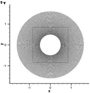
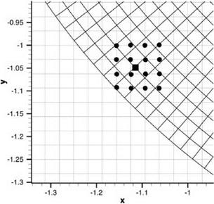 Figure 13.5. Interpolation from a Cartesian grid to a polar grid using a 16-point stencil. Ax = Ay = Ar = 1/32.
Figure 13.6. A 16-point irregular interpolation stencil.
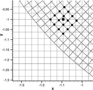
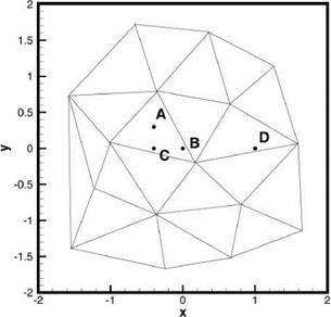 The development of optimized multidimensional interpolation is, in many respects, similar to that in one dimension. Consider an interpolation stencil in a computational domain as shown in Figure 13.6. Without loss of generality, the interpolation is considered for implementation in the x – y plane. However, x and y may be a set of curvilinear coordinates in the physical domain. For interpolation purposes, the values of a function f(x, y) are given at the stencil points (x, y), j = 1,2,…, N for an N-point stencil. The objective is to estimate the value f(xo, yo) at a general point P at (xo, yo). By definition of interpolation (not extrapolation), the point P lies within the boundary of the stencil as defined by Figure 13.6. Let dj be the distance between neighboring points of the stencil. A useful length scale is
1 K
A = – J2 dj. (13.3)
j=1
where K is the number of links between stencil points.
The most general interpolation formula in two dimensions has the following form:
N
f (xo. Уо) = Y^ Sjf (xj > yj )• (13.4)
j=1
Different interpolation methods determine the coefficient Sj in different ways.
It will be assumed that the function f(x, y) to be interpolated has a Fourier inverse transform, such that
TO TO
f(X. y) = ft«.e)e»+ey>d«de. (13’5)
-TO – TO
where (а, в) are the wave numbers in the x and y directions, respectively.
Let A(a, в) = | f (а, в)| and ф(а, в) = arg[f (а, в)], Eq. (13.5) maybe rewritten
w w
f {x-» = f ІА(а-в)Є’‘х+п^а (136)
This equation may be interpreted in the sense that f(x, y) is made up of a superposition of simple waves exp[i(ax + by + ф(а, b))] with amplitude A(a, в). It is useful to define the local interpolation error, Elocal, for wave number (а, в) as the absolute value of the difference between the left and right side of Eq. (13.4) when f(x, y) is replaced by the simple wave as follows:
Here all simple waves are assumed to have unit amplitude; i. e., А(а, в) = 1.0. It is easy to find as follows:
N
■ j = 1
The total error, E, over the region – к < аД, вД < к, in wave number space is
 |
||||||
obtained by integrating Efocal of Eq. (13.8) over this region, i. e.,
When the function to be interpolated is a constant, which corresponds to setting а = в = 0 in Eq. (13.7), it is reasonable to require the local interpolation error to be zero. By Eq. (13.8), this requirement leads to
N
 ES; -1 = 0
j=1
 |
|
It is now proposed that the interpolation coefficients, Sj (j = 1, 2,…, N) be chosen such that E2 is a minimum subjected to constraint (13.10). This can readily be done by using the method of the Lagrange multiplier. Let
where k is the Lagrange multiplier. The conditions for L to be a minimum are
dL = 0, dL = 0, j = 1,2,…,n. (13.12)
It is easy to find that the condition dL/дSj = 0 yields
where Re{} is the real part of {}. Similarly it is easy to find that 9L/дк leads to
N
![]() ESj -1 = 0
ESj -1 = 0
which is constraint (13.10).
Eqs. (13.13) and (13.14) form a linear matrix system of (N + 1) unknowns for Sj (j = 1,2,…, N) and к. It turns out that all the integrals of Eq. (13.13) can be evaluated in closed form. This allows the matrix elements to be written out explicitly. The values of Sj may be found by solving the matrix system as follows:
AS = b, (13.15)
 |
 |
where vector ST = (S1 S2 S3 … SN к). Note: Superscript T denotes the transpose. The elements of the coefficient matrix A and vector b are given by
Note: In the case Xj = Xk and/or yj = yk or Xj = X0 or yj = y0 the limit forms of these formulas are to be used. Computationally, the limit forms are used wherever |Xj – xk| < c or |yj – yk| < c. This is discussed in Appendix 13A at the end of of this chapter.
It is useful to point out that Ajk depends on A and К as well as the coordinates of the stencil points only. The coordinates of the point to be interpolated to, (x0, y0), appears only in bj. Thus, if many values of f are to be interpolated using the same stencil, A and A-1 need only be computed once.
For error estimate purposes, the following symmetry properties of the local error, given by Eq. (13.8), can easily be derived.
![]() £local (а, в) = Elocal (-a> – У Elocal (-а, в) = Elocal (a> -в) .
£local (а, в) = Elocal (-a> – У Elocal (-а, в) = Elocal (a> -в) .
Thus, once S/s are found, Elocal can be calculated by formula (13.8). Upon invoking Eqs. (13.22) and (13.23), it is sufficient to examine Elocal(a, в) over the upper half of the aA – в A plane for – п < а А, в A < п.
![]() Computationally, there are two general ways to treat problems with complex geometry. One way is to use unstructured grids. The other is to use overset grids. Overset grids are formed by overlapping structured grids. In this chapter, the basic idea of overset grids methodology and its implementation are discussed.
Computationally, there are two general ways to treat problems with complex geometry. One way is to use unstructured grids. The other is to use overset grids. Overset grids are formed by overlapping structured grids. In this chapter, the basic idea of overset grids methodology and its implementation are discussed.
13.1 Basic Concept of Overset Grids
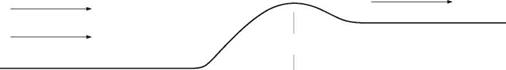
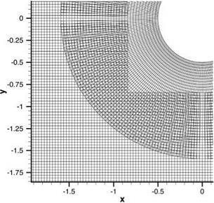
To illustrate the basic idea of overset grids, consider the problem of computing the scattering of acoustic waves by a solid cylinder in two dimensions. In the space around the cylinder, the coordinates of choice for computing the solution is the cylindrical polar coordinates centered at the axis of the cylinder. This coordinate system provides a set of body-fitted coordinates and, hence, a body-fitted mesh when discretized around the cylinder. One significant advantage of using a body-fitted grid is the relative ease in enforcing the no-through-flow wall boundary condition using the ghost point method or other methods. Away from the cylinder, acoustic waves propagate with no preferred direction. The natural coordinate system to use is the Cartesian coordinates. Therefore, to take into account the advantages stated, one may use a polar mesh around the cylinder and a Cartesian mesh away from the cylinder with an overlapping mesh region. The overlapping mesh region is for data transfer from one set of grids to the other and vice versa.
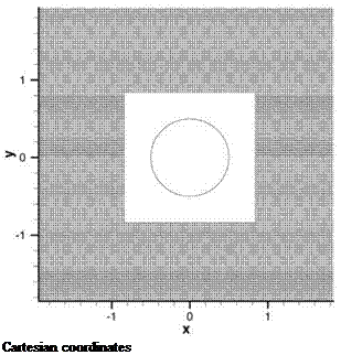
Figure 13.1 shows a Cartesian mesh with a square hole around the cylinder. For the purpose of putting all variables in dimensionless form, the diameter, D, of the cylinder is taken as length scale, speed of sound a0 as the velocity scale, D/a0 as the time scale, p0 (the density of the undisturbed gas) as the density scale, and p0a2 as the pressure scale. The mesh size is Ax = Ay = 1/32. The size of the square hole is 1.6 by 1.6. Figure 13.2 shows a polar mesh with Ar = 1/32 and Ав = n/150. The polar mesh extends to a distance of r = 1.5. The mesh overlap region is between the square and the outside edge of the polar mesh as shown in Figure 13.2. Figure 13.3 is an enlarged view of the mesh overlap region. Both the cylindrical mesh and the Cartesian mesh are structured meshes. To compute the solution, it would be best to write the governing equations in the coordinate system used. For acoustic wave scattering problems under discussion, the governing equations are the full Euler equations. In dimensionless form, they are
 |
||
 |
Figure 13.1. Cartesian grid used in acoustic wave scattering by a cylinder problem.
Figure 13.3. The overlapping region of the Cartesian and polar grids.
 Polar coordinates
 dp 1 d
— +——— (pvrr) + —
dt r 9r r r d0
9 vr 9 vr v- 9 vr v2 1 9p
—- + v—- + ———— —— + = 0
dt r 9r r d – r p 9r
9 v – 9 v – v – 9 v – vrv – 1 9 p
– + vr – + – – + r- – + = 0
dt r 9r r d0 r pd0
![]() 9 p 9 p vRd p (1 9 vrr 1 9 vfl 0
9 p 9 p vRd p (1 9 vrr 1 9 vfl 0
+ vr + – + Y p r + – = 0.
dt r 9r r d0 r 9r r d0
The solution of (13.1) is computed on the Cartesian mesh. The solution of (13.2) is computed on the polar mesh. (u, v) and (vr, v-) are related by
u = vr cos – – v – sin – v = vr sin – + v – cos – vr = u cos – + v sin-. v- = – u sin – + v cos –
In computing the solution, the 7-point stencil dispersion-relation-preserving (DRP) scheme may be used. Since the 7-point stencil DRP scheme is a central difference scheme, the values of the computation variables of the three rows and columns of the Cartesian mesh around the square hole are not computed by the time marching scheme. They are found by interpolation from the values of the polar mesh using, say, a 16-point regular stencil. A typical stencil is shown in Figure 13.4. For the polar mesh, the values of the computation variables at the outer three rings are not computed. They are interpolated from the values of the Cartesian mesh using a 16-point regular stencil as shown in Figure 13.5.
Data transfer from one set of grids to the other is one of the crucial processes of the overset grids method. Since a high-resolution scheme is used for computation in each of the structured grids, it is important for the data transfer process to retain
Figure 13.4. Interpolation from a polar grid to a Cartesian grid using a 16-point stencil. Ax = Ay = Ar = 1/32, A0 = n/150.
 at least the same accuracy. In what follows, a highly accurate multidimensional interpolation scheme, suitable for use as a data transfer method, is discussed.
When high-quality, high-order computations are to be performed, one expects that large derivative stencils are to be used in the mesh-size-change buffer region. Optimized coefficients of several large buffer stencils are listed below. n is the range of optimization.
9-Point Stencils
1357 derivative stencil. n = 0.885, a0 = 0.0
al = —a-1 = 0.6090238560979105951878503463135849 a3 = — a—3 = —0.04690263734690552411752317530947456 a5 = —a—5 = 7.45976157440795270904970345070725E-3 a7 = — a—7 = —8.021074184619694829327625198139366E-4
1246 derivative stencil. n = 1.075, a0 = 0.0
al = —a—1 = 0.7512246907952941262715227576491948 a2 = —a—2 = —0.1390991789681719362022172210597338 a4 = —a—4 = 7.6185409515963687179825703762642764E-3 a6 = —a—6 = —5.834161108892881231697661724640704E-4
1235 derivative stencil. n = 1.215, a0 = 0.0
al = —a—1 = 0.8080701723801081268126989813400916 a2 = —a—2 = —0.2043432375248032483484509202108968
11-
 |
Point Stencils
13579 derivative stencil. n = 0.96, a0 = 0.0
a3 = – a-1 = 0.6169610748807038603650623876266686 a3 = – a-3 = -0.053037977159713435091000295888159493 a5 = – a-5 = 0.011057680967517392356513295707997069 a7 = – a-7 = -2.2180071199244495954136156095099006E-3 a9 = – a-9 = 2.6561128892451447702970341826597076E-4 12468 derivative stencil. n = 1.15, a0 = 0.0
a3 = – a-1 = 0.7631614437828716630397535144418575 a2 = – a-2 = -0.14840307207850050785201259674573818 a4 = —a-4 = 0.010272925705412492924195271253581683 a6 = — a—6 = —1.4476431210717408970741183395007183E-3 a8 = —a—8 = 1.54857034863728293741913009037069E-4
12357 derivative stencil. n = 1.3, a0 = 0.0
ax = —a—1 = 0.8252543028344873666308890959218707 a2 = — a—2 = —0.2230034607664662190128310868797273
a3 = – a-3 = 0.0434847322758841815894783782752433 a5 = – a-5 = -2.167191168162797315544034817529481E-3 a7 = – a-7 = 1.6205395880093045772258815707159745E-4
12346 derivative stencil. n = 1-4, a0 = 0.0
a3 = – a-1 = 0.8559670270533940785913013975770142 a2 = – a-2 = -0.26355038029346495866745731339388584 a3 = – a-3 = 0.07259552278997621476486631628514457 a4 = —a—4 = -0.012148236925938859899155655963543882 a6 = —a—6 = 3.2335214456043900760615070158323756E-4
13-Point Stencils
1357911 derivative stencil. n = 1.04, a0 = 0.0
a3 = —a—1 = 0.6222744810884503208006161752402352 a3 = —a—3 = —0.05745752283507652911500016054804188 a5 = —a—5 = 0.014048807353574197207816006070727958 a7 = —a—7 = —3.8223706624986957120774761605838786E-3 a9 = —a—9 = 8.773256282094535158374388508297744E-4 an = —a—u = —1.1684412431690283206275822573907119E-4
1246810 derivative stencil. n = 1.225, a0 = 0.0
a3 = —a—1 = 0.7704159669204072987577907570660112 a2 = —a—2 = —0.15423090409941798512572684114924175 a4 = —a—4 = 0.012111428866866974752283356866705977 a6 = — a—6 = —2.237909249412284471498739008161985E-3 a8 = —a—8 = 4.5510386970466766460616813555659377E-4 a10 = — a—10 = —6.132496502028620033274132698325002E-5
123579 derivative stencil. n = 1.375, a0 = 0.0
a3 = —a—1 = 0.8346007521198306780385577274355369 a2 = — a—2 = —0.23351453982173775751336583621371804 a3 = —a—3 = 0.048416204296670338536750729561625173 a5 = —a—5 = —3.0732634681711003723284703258379413E-3 a7 = —a—7 = 4.2764556235837229592649414282684104E-4 a9 = —a—9 = —4.972077355769809243570567373051316E-5
123468 derivative stencil. n = 1.5, a0 = 0.0
a3 = —a—1 = 0.8695040147146564312615709824565512 a2 = —a—2 = —0.28111202563583404799569450627628445
a3 = – a-3 = 0.0845286783216550621158838448960038 a4 = – a-4 = -0.01627930669247656566519371821994323 a6 = -a-6 = 7.921732807092020750043354094040387E-4 a8 = —a—8 = -6.272641528780892588558052108063413E-5
123457 derivative stencil. n = 1.59, a0 = 0.0
ax = —a—1 = 0.8891744805205031441686220773749192 a2 = – a-2 = -0.3096468670894452798278980518929917 a3 = – a-3 = 0.10899054209331996393360155629344859 a4 = —a—4 = -0.030279357225089779657034797121953563 a5 = —a—5 = 5.0487756298281625592780951771430825E-3 a7 = — a—7 = —1.3983169576488149741170426674042277E-4
15-Point Stencils
135791113 derivative stencil. n = 1.11, a0 = 0.0
a3 = —a—1 = 0.6258779354573266902120076920113189 a3 = —a—3 = —0.060595621262294137510257150629882345 a5 = —a—5 = 0.016419419315514504253832969339583166 a7 = —a—7 = —5.332041836769511268442174297083009E-3 a9 = —a—9 = 1.6673308740708772699299319145046008E-3 au = —a—11 = —4.2649198385963323058082868711331986E-4 a13 = — a—13 = 6.31968127067576950549124298229811E-5
124681012 derivative stencil. n = 1.295, a0 = 0.0
a3 = —a—1 = 0.7751653818251308369767154456316511 a2 = —a—2 = —0.15810842159142594570323780970792248 a4 = —a—4 = 0.01344368848930721405861880589370375 a6 = — a—6 = —2.882509303736270724294138583564854E-3 a8 = —a—8 = 7.737358357276028905705620340672378E-4 a10 = — a—10 = —2.0178401810068388499797391894808376E-4 a12 = —a—12 = 3.3309726507986522205418718975874384E-5
12357911 derivative stencil. n = 1.45, a0 = 0.0
a3 = —a—1 = 0.8405083211561195585119035254044648 a2 = —a—2 = —0.24028234117501536764416518113371986 a3 = —a—3 = 0.051710722871922495965649571941564053 a5 = — a—5 = —3.7380739291593315864384143663748303E-3 a7 = —a—7 = 6.732308091610869543962441130822362E-4 a9 = -a-9 = -1.521289737983841685480415909565809E-4 au = – a-11 = 2.464612036347233162080530883553833E-5
12346810 derivative stencil. n = 1-58, a0 = 0.0
a1 = – a-1 = 0.8769697517162914222723512564100425 a2 = —a-2 = -0.2910485506050849365005963442595554 a3 = —a—3 = 0.09160729636798243850623886924431454 a4 = — a—4 = —0.018889586310816595242600622281686327 a6 = —a—6 = 1.1725375731033384971390388407682345E-3 a8 = — a—8 = —1.7648972164255100846899103703416032E-4 a10 = — a—10 = 2.404979677178932654450087545336078E-5
1234579 derivative stencil. n = 1.69, a0 = 0.0
al = —a—1 = 0.8996669663763338312112615547268505 a2 = —a—2 = —0.3248239503161405595421655578148774 a3 = —a—3 = 0.12185450769709449174616083733794719 a4 = — a—4 = —0.03732240294041507819400704949257943 a5 = —a—5 = 7.198430554922608039998318584879614E-3 a7 = —a—7 = —3.6954649492803779167797176495157803E-4 a9 = —a—9 = 3.3521735134149972485495143293701953E-5
1234568 derivative stencil. n = 1.765, a0 = 0.0
a3 = —a—! = 0.9132066730017018501071844317880848 a2 = —a—2 = —0.3458970880904337489997562609890365 a3 = —a—3 = 0.1423752402318168875470781806014907 a4 = —a—4 = —0.051759351567246811093075274001630856 a5 = —a—5 = 0.01455611850194688853308973731674671 a6 = —a—6 = —2.4817385325786229531655586408536866E-3 a8 = —a—8 = 7.612842980494058461741370667849726E-5
12.5 Large Buffer Selective Damping Stencils
Buffer regions, where a change in mesh size takes place, are favorite sites for the generation of spurious short numerical waves. These are also regions prone to numerical instability. It is, therefore, necessary to add artificial selective damping to these regions. Below are optimized coefficients of several large artificial selective damping stencils designed for use in buffer regions involving change in mesh size by a factor of 2.
9-Point Stencil. a = 0.1975n
1235 stencil. в = 1.215
d0 = 0.2708886738189505 d1 = d_1 = -0.2206703054137707 d2 = d-2 = 0.11455566309052476 d3 = d-3 = -0.031235919680725313 d5 = d-5 = 2.5094190624960092E-3
1246 stencil. в = 1.075
d0 = 0.33027355532845215 d1 = d-1 = -0.25 d2 = d-2 = 0.09475341549663605 d4 = d-4 = -0.011705918179843176 d6 = d-6 = 1.815725018981057E-3
1357 stencil. в = 0.885
d0 = 0.5
dx = d-1 = -0.3062891172075045 d3 = d-3 = 0.07419885992060947 d5 = d-5 = -0.022186172045155307 d7 = d-7 = 4.276429332050351E-3
11-Point Stencil. a = 0.195n
13579 stencil. в = 0.96
d0 = 0. 5
dx = d-1 = -0.3095004246385787 d3 = d-3 = 0.08211616467055119 d5 = d-5 = -0.03036277454777355 d7 = d-7 = 9.650309477159707E-3 d9 = d-9 = -1.9032749613586592E-3
12468 stencil. в = 1.15
d0 = 0.32646005443343434 d1 = d-1 = -0.25 d2 = d-2 = 0.09831710703893635 d4 = d-4 = -0.014318492283620247 d6 = d-6 = 3.4468599861078082E-3 d8 = d-8 = -6.755019581410823E-4
12357 stencil. в = 1-3
d0 = 0.2635716529562409 d1 = d_1 = -0.21772629224768608 d2 = d_2 = 0.11821417352187955 d3 = d_3 = -0.03499568161296116 d5 = d_5 = 3.174478225315305E-3 d7 = d_7 = -4.5250436466805904E-4
12346 stencil. в = 1.4
d0 = 0.23453190899565207 dx = d_! = _0.19992274952791061 d2 = d_2 = 0.12196569374380435 d3 = d_3 = _0.050077250472089385 d4 = d_4 = 0.011317101840646436 d6 = d_6 = _5.487500822768231E-4
13-Point Stencils. a = 0.1925n
1357911 stencil. в = 1.04
d0 = 0. 5
dx = d_! = _0.31182671961098623 d3 = d_3 = 0.08793722059177961 d5 = d_5 = _0.037310514270787353 d7 = d_7 = 0.015220028715708166 d9 = d_9 = _5.094690254969648E-3 d11 = d_11 = 1.0746748292554631E-3 1246810 stencil. в = 1.225
d0 = 0.3240020968562207 d1 = d_x = _0.25 d2 = d_2 = 0.10058161761678362 d4 = d_4 = _0.016211394630950087 d6 = d_6 = 4.751848956897231E-3 d8 = d_8 = _1.4728623391755445E-3 d10 = d_10 = 3.497419683344133E-4 123579 stencil. в = 1.375
d0 = 0.2595758998570965
d1 = d_! = _0.2161210442492141
d2 = d-2 = 0.12021205007145175 d3 = d-3 = -0.037173351241118195 d5 = d-5 = 3.961825142400804E-3 d7 = d-7 = -8.500469444013784E-4 d9 = d-9 = 1.8261729233287355E-4
123468 stencil. в = 1.5
d0 = 0.22856643029671658 dx = d-1 = -0.19658662660320927 d2 = d-2 = 0.12336415951962278 d3 = d-3 = -0.053413373396790725 d4 = d-4 = 0.01316893300174682 d6 = d-6 = -9.489310483476328E-4 d8 = d-8 = 1.3262337861974504E-4
123457 stencil. в = 1.59
d0 = 0.21457119275070027 d3 = d-1 = -0.18683026262805987 d2 = d-2 = 0.12266004527546252 d3 = d-3 = -0.05945584021704768 d4 = d-4 = 0.020054358349187353 d5 = d-5 = -3.8748982424400496E-3 d7 = d-7 = 1.610010875476098E-4
15-Point Stencils. a = 0.19n
135791113 stencil. в = 1.11
d0 = 0.5
d3 = d-1 = -0.31339818418385334 d3 = d-3 = 0.0921696857561028 d5 = d-5 = -0.042740680643837763 d7 = d-7 = 0.020359003550007293 d9 = d-9 = -8.78888052362071E-3 d11 = d-11 = 3.1146836013276404E-3 d13 = d-13 = -7.156275561259213E-4
124681012 stencil. в = 1.295
d0 = 0.32236714053321097
dx = d-x = -0.25
d2 = d-2 = 0.10216769227713358
d4 = d-4 = -0.01756253154787246 d6 = d-6 = 5.840424337495861E-3 d8 = d-8 = -2.2168366108895102E-3 d10 = d-10 = 8.252438932473476E-4 d12 = d-12 = -2.3756261572031736E-4
12357911 stencil. в = 1.45
d0 = 0.25689444748256046 dt = d-1 = -0.21501278581108324 d2 = d-2 = 0.12155277625871977 d3 = d-3 = -0.038648799797586175 d5 = d-5 = 4.562916765604436E-3 d7 = d-7 = -1.1632920312828478E-3 d9 = d-9 = 3.7616806999180853E-4 du = d-u = -1.1420719564397982E-4
12346810 stencil. в = 1.58
d0 = 0.22513862785383467 dt = d-1 = -0.1946531938734711 d2 = d-2 = 0.12416686947715667 d3 = d-3 = -0.0553468061265289 d4 = d-4 = 0.014280517691395201 d6 = d-6 = -1.1996097976025642E-3 d8 = d-8 = 2.4498737887899095E-4 d10 = d-10 = -6.207867674562712E-5
1234579 stencil. в = 1.69
d0 = 0.21047015796352988 dx = d-1 = -0.18421029309503222 d2 = d-2 = 0.12295164373519486 d3 = d-3 = -0.06145360873722441 d4 = d-4 = 0.02181327728304021 d5 = d-5 = -4.569637725373214E-3 d7 = d-7 = 2.7404296254122305E-4 d9 = d-9 = -4.050340491136648E-5
1234568 stencil. в = 1.765
d0 = 0.20494238199107911 dx = d-1 = -0.1800055838379142
![]()
|
|
|
|
![]()
d2 = d-2 = 0.12179720514762138 d3 = d-3 = -0.06311640230450315 d4 = d-4 = 0.024628464984657864 d5 = d-5 = -6.878013857582646E-3 d6 = d-6 = 1.1454459542189518E-3 d8 = d-8 = -4.2307082037753E-5
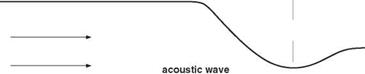
EXERCISES 12.1. In a transonic cascade, the local Mach number of the flow in the narrow passages may be close to sonic. The computation of sound propagating through such regions presents a challenging problem. To reduce the complexity of the problem, but retaining the basic physics and difficulties, a one-dimensional acoustic wave transmission problem through a nearly choked nozzle is considered.
The following characteristic scales are used to form dimensionless flow variables.
length scale = diameter of nozzle in the uniform region downstream of the throat (see Figure 12.22), D
velocity scale = speed of sound in the same region, aTO time scale = D/a
density scale = mean density of gas in the same region, pTO pressure scale = p^a2^
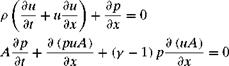
Consider a one-dimensional nozzle with an area distribution as follows:
= j 0.536572 – 0.198086e-(ta2)(x/0’6)2, x > 0 X = 1.0 – 0.661514e-(ln2)(x/0’6)2, x < 0 ‘
The governing equations in dimensionless form are
dp 1 dpuA dt A dx
|
|
where y = 1.4. The Mach number in the uniform region downstream of the throat is 0.4.
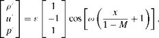
Small-amplitude acoustic waves, with angular frequency ы = 0.6 n, are generated way downstream and propagate upstream through the narrow passage of the nozzle throat. Let the upstream propagating wave in the uniform region downstream of the nozzle throat be
|
|
where с = 10-5. Use a computation domain of size 20,10 upstream and 10 downstream of the nozzle throat, to calculate the distribution of maximum acoustic pressure inside the nozzle.
This problem can, of course, be calculated accurately if a very large number of mesh points is used. But this is not always practical. It is recommended that no more than 400 mesh points be used. In other words, use a multisize mesh to compute the solution. The boundary conditions developed in Problem 6.5 would be useful, as well.
The exact solution of this problem is available in the Proceedings of the Third Computational Aeroacoustics Workshop on Benchmark Problems, NASA CP-2000209790, August 2000.
Artificial selective damping is added to the time marching DRP scheme to eliminate spurious short waves and to prevent the occurrence of numerical instability. The damping stencil with a damping curve of half-width 0.2n is used for background damping. Near the solid walls or the outer boundaries where a 7-point stencil does not fit, a 5- or 3-point stencil as provided in Section 7.4 is used instead. For general background damping, an inverse mesh Reynolds number of 0.05 is used everywhere. Along walls and mesh-change interfaces, additional damping is included. The added damping has an inverse mesh Reynolds number distribution in the form of a Gaussian function with the maximum value at the wall or interface and a half-width of 4 mesh points as in the first example. On the wall, the maximum value of R^1 is set equal to 0.15. The corresponding value at a mesh-size-change interface is 0.3. There are three external corners at the cavity opening. They are probably sites at which short spurious waves are generated. To prevent numerical instability from developing at these points, additional artificial selective damping is imposed. Again, a half-width of 4 mesh point Gaussian distribution of the inverse mesh Reynolds number centered at each of these points is used. The maximum value of R^1 at these points is set equal to 0.35. By implementing artificial selective damping distribution as described, no numerical instability nor excessive short spurious waves have been found in all the computations.
12.4.2.2 Numerical Results
To start the computation, the time-independent boundary layer solution without the cavity is used as the initial condition. The solution is time-marched until a time periodic state is reached.
The characteristic features of the flow in the vicinity of the cavity opening and the acoustic field are found by examining the instantaneous vorticity, steamlines, and pressure contours. Figure 12.16 shows a plot of the instantaneous vorticity contours for the case U = 50.9 m/s and 5 = 2.0 mm. As can easily be seen, vortices are
Figure 12.16. Instantaneous vorticity contours showing the shedding of small vortices at the trailing edge of the cavity. U = 50.9 m/s, S = 2 mm.
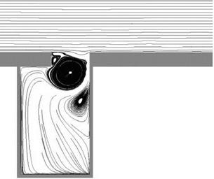
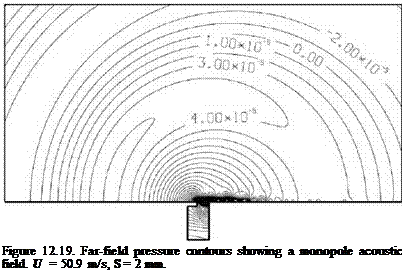
 shed periodically at the trailing edge of the cavity. Some shed vortices move inside the cavity. Other vortices are shed into the flow outside. The shed vortices outside are convected downstream by the boundary layer flow. These convected vortices are clearly shown in the pressure contour plot of Figure 12.17. They form the low- pressure centers. These vortices persist over a rather long distance and are eventually dissipated by viscosity. Figure 12.18 shows the instantaneous streamline pattern. It is seen that the flow at the mouth of the cavity is completely dominated by a single large vortex. Below the large vortex, another vortex of opposite rotation often exists. The position of this vortex changes from time to time and does not always attach to the cavity wall. The near-field pressure contour pattern is shown in Figure 12.19. This pattern is the same as that of a monopole acoustic source in a low subsonic stream. That the noise source is a monopole, and not a dipole, is consistent with the model of Tam and Block (1978). The sound is generated by flow impinging periodically at the trailing edge of the cavity.
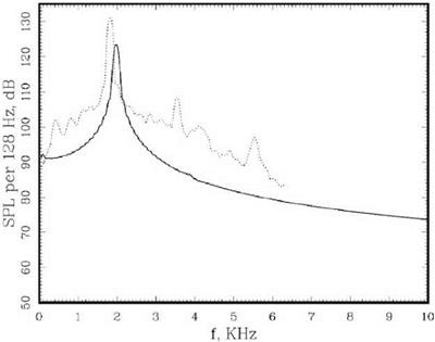
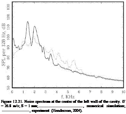
Experiments indicate that cavity resonance may consist of a single tone or multiple tones. The number of tones occured depend on the flow conditions and the cavity geometry. Figure 12.20 shows the noise spectrum measured at the center of the left wall of the cavity at U = 50.9 m/s, S = 2 mm. The spectrum consists of a single tone at 1.99 kHz.
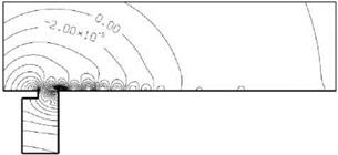 Figure 12.17. Near-field pressure contours showing the convection of shed vortices along the outside wall. U = 50.9 m/s, S = 2 mm.
Figure 12.18. Instantaneous streamline pattern. U = 50.9 m/s, S = 2 mm.
Shown in Figure 12.20 also is the spectrum measured experimentally by Henderson (2000). There is good agreement between the tone frequency of the numerical simulation and that of the physical experiment. In the experiment, the boundary layer is turbulent; therefore, it is not expected that there would be good agreement in the tone intensity. Figure 12.21 shows the noise spectrum at the lower speed U = 26.8 m/s and S = 1 mm. In this case, there are two tones. One is at a frequency of 1.32 kHz and the other at 2.0 kHz. This is in fair agreement with the experimentally measured spectrum. Again, the tone frequencies are reasonably well reproduced in the numerical simulation, but the tone intensities are different. Figures 12.20 and 12.21 together suggest that as the flow velocity increases, one of the tones disappears. The strength of the remaining tone intensifies with flow speed.
|
Figure 12.20. Noise spectrum at the center of the left wall of the cavity. U = 50.9 m/s; S = 2 mm; , numerical simulation; , experiment (Henderson, 2004). |
The governing equations are the compressible Navier-Stokes equations in two dimensions. In dimensionless form with D(D = 3.3 mm is the thickness of the cavity overhang) as length scale, U, the free-stream velocity (from left to right), as velocity scale, D/U as the time scale, p0, the ambient gas density, as the density scale and p0U2 as the pressure scale, they are
|
dp 9Uj dp + p + и j = 0 91 H dXj 1 dXj |
(12.37) |
|
9и 9и _ dp dtij “I – U — “Idt 19 Xj 9 xt 9 Xj |
(12.38) |
|
9 p 9 p 9 Uj It + и1 Ц + Y p dXj = 0 |
(12.39) |
|
T = _jl + дииЛ 4 Rd dxj dxi |
(12.40) |
where Rd is the Reynolds number based on D.
These equations are solved in time by the multi-size-mesh multi-time-step DRP algorithm. In each subdomain of Figure 12.15, the equations are discretized by the DRP scheme. At the mesh-size-change boundaries, special stencils as given in
Section 12.1 are used. The time steps of adjacent subdomains differ by a factor of 2 just as the mesh size does. With the use of the multi-size-mesh multi-time-step algorithm, most of the computation effort and time are spent in the opening region of the cavity where the resolution of the unsteady viscous layers is of paramount importance.
12.4.2.1 Numerical Boundary Conditions
Along the solid surfaces of the cavity and the outside wall, the no-slip boundary condition is enforced by the ghost point method. Along the vertical external boundary regions (3 mesh points adjacent to the boundary), the flow variables are split into a mean flow and a time-dependent component. The mean flow, with a given boundary layer thickness, is provided by the Blasius solution. The time-dependent part of the solution is the only portion of the solution that is computed by the time marching scheme. The boundary conditions used for the computation are as follows. Along the top and left external boundaries, the asymptotic radiation boundary conditions of Section 6.1 are imposed. Along the right boundary, the outflow boundary conditions of Section 9.3 are used.
The computation domain is shown in Figure 12.15. It is designed primarily for the case U = 50.9 m/s and a boundary layer thickness 5 = 2 mm. In the cavity opening region, viscous effects are important. To capture these effects, a fine mesh is needed. Away from the cavity, the disturbances are mainly acoustic waves. By using the DRP scheme in the computation, only a very coarse mesh would be necessary in the acoustic region. The mesh design is dictated by these considerations. The computation domain is divided into a number of subdomains as shown in Figure 12.15. The finest mesh with Ax = Ay = 0.0825 mm is used in the cavity opening region. The mesh size increases by a factor of 2 every time one crosses into the next subdomain. The mesh size in the outermost subdomain is thirty-two times larger than the finest mesh.
|
Figure 12.15. Computational domain showing the division into subdomains and their mesh size. D = 3.3 mm. |
This problem is to compute the resonance tones induced by a turbulent boundary layer flow outside a scaled model automobile door cavity. To properly model and compute the turbulent boundary layer flow and its interaction with the cavity is a task that will require extensive time and effort. Here, a laminar boundary layer is considered instead. It is believed that the cavity tone frequencies would most likely be about the same whether the flow is turbulent or laminar, but the tone intensities are expected to be different.
A boundary layer flow will definitely be laminar if Rs* < 600. Rs* is the Reynolds number based on the displacement thickness. This is the Reynolds number below
, asymptotic.
the stability limit of the Tollmien-Schlichting waves. In modern facilities with low free-stream turbulence and sound, a boundary layer may remain laminar if Rs* is larger than 600, but less than 3400. For a free-stream velocity of 50.9 m/s and 26.8 m/s (velocities prescribed by the benchmark problem), these correspond to a boundary layer thickness of 2.9 mm and 5.5 mm, respectively. In this example, consideration will be restricted to boundary layer thicknesses of 2 mm and 1 mm at flow velocities of 50.9m/s and 26.8m/s, respectively.
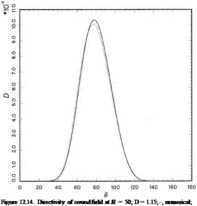
An asymptotic solution of the present problem may be found by a straightforward application of Fourier transform. Details of the analysis are given in the Proceedings of the Third CAA Workshop on Benchmark Problems (NASA CP-2000-209790, August 2000; Dahl, M. D. ed.). The directivity of sound radiation with respect to a spherical polar coordinate system (R, в, ф) with the polar axis coinciding with the axis of the rotor is
![]()
Lim R2p2
12.4.1.5 Numerical Results
Eqs. (12.34) are discretized according to the multi-size-mesh mult-time-step DRP scheme and marched in time to a time periodic state. To start the computation, a zero initial condition is used. Figure 12.13 shows a comparison of the directivity at
|
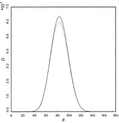
Figure 12.13. Directivity of sound field at R = 50; D = 0.85;– , numerical;….. , asymptotic. |
R = 50 obtained computationally against the asymptotic solution for D = 0.85, the subsonic tip speed case. As expected, most of the acoustic radiation is concentrated in the plane of rotation. There is good agreement between the numerical results and the asymptotic solution. Figure 12.14 shows the directivity at supersonic tip speed with D = 1.15. At higher frequency, the acoustic wavelength is shorter. This case, therefore, offers a more stringent test of the accuracy of the entire computational algorithm. The agreement with asymptotic solution is reasonably good.