Our heavyweight helicopter equal in the world does not have
In Rostov started production of the most load-lifting rotary-wing car The Russian holding «Helicopt[...]

Everything about aircrafts and helicopters. News and events in aviation worldwide. Civil, transportation, military helicopters and airplanes.

Everything about aircrafts and helicopters. News and events in aviation worldwide. Civil, transportation, military helicopters and airplanes.

Everything about aircrafts and helicopters. News and events in aviation worldwide. Civil, transportation, military helicopters and airplanes.

Everything about aircrafts and helicopters. News and events in aviation worldwide. Civil, transportation, military helicopters and airplanes.


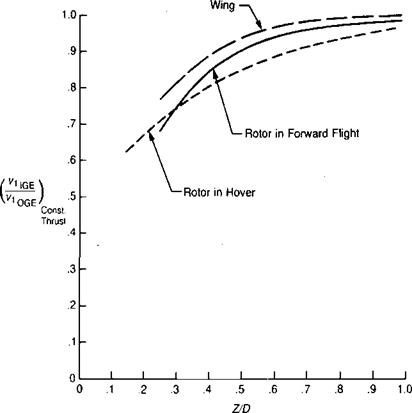
In forward flight the rotor obtains a beneficial effect from flying near the ground, just as it does in hover. The ground effect may be expressed in terms of the ratio of the induced velocity in and out of ground effect. This ratio has been determined for a rotor from the work of reference 3.10 and is plotted in Figure 3.10. Also shown is the same ratio for a wing from reference 3.11 and for a hovering rotor from Figure 1.41 of Chapter 1. Note the similarity of all three curves. The induced power required is proportional to the induced velocity ratio and thus is reduced for flight near the ground. If the ratio applied at all flight conditions, it could be concluded that the induced power would always decrease as the helicopter went from hover to forward flight near the ground as well as away from the ground.
|
FIGURE 3.10 Effect of Ground on Induced Velocity Ratios in Forward Flight and in Hover |
Source for rotor in forward flight: Heyson, “Ground Effect for Lifting Rotors in Forward Flight," NASA TND-234,1960; for rotor in hover: Figure 1.41; for wing: Hoak, "USAF Stability and Control DATCOM,” 1960.
Test experience, however, shows that during transition from hover to forward flight at heights less than about half the rotor diameter, the power may actually increase rather than decrease. Pilots speak of this as "running off the ground cushion.” Figure 3.11 shows the effect as measured in flight and reported in reference 3.12 and in a wind tunnel from reference 3.13. The reversal of ground effect is due to the helicopter overrunning the ground vortex, as illustrated in Figure 3-12, which is based on the wind tunnel observations of reference 3.13. As the leading edge of rotor approaches the ground vortex, the inflow is increased just as if part of the rotor were in a climb, thus increasing the power required. The recovery to a more normal inflow pattern occurs suddenly as the vortex passes under the rotor. The effect of the ground vortex on tail rotor performance in sideward and rearward flight is discussed in references 3.1 and 3.14.
The characteristics of the power required equations make it possible to easily calculate the power required at altitude if the power required at sea level at several gross weights has already been determined. Assuming that the main rotor thrust is equal to the gross weight, the main rotor power equation may be rewritten:
G. W.
P/Po
l,100p 0AVe 1,100
 |
 |
and the equation for the tail rotor power in the same form is:
The form of these equations shows that for calculating purposes, weight and density do not have to be treated as separate variables, but that one set of calculations made at sea level at several gross weights can also be used for altitude calculations. For example, Figure 4.38 of Chapter 4 shows the power required by the example helicopter at sea level at several gross weights. To obtain the power required at altitude, the gross weight is divided by the density ratio and the gross weight curve corresponding to this equivalent weight is used. The corresponding values of equivalent power read from the curves are multipled by the density ratio to obtain the actual power.
This method is valid except in those cases where compressibility effects on profile power are significant. Since these effects are a function of temperature
rather than of density ratio, they will have to be estimated separately, by methods discussed in a later section.
The tail rotor power can be analyzed with the same approximations used for the main rotor. The tail rotor thrust required to balance the main rotor thrust is:
where the subscript, M, applies to the main rotor and lT is the tail rotor moment arm with respect to the main rotor shaft. The tail rotor is not used to overcome drag, so its equation has no parasite power term as the main rotor does. To a first approximation, the tail rotor power in forward flight is:
![]()
![]() where the subscript, T, indicates that all physical parameters are those of the tail ‘ rotor.
where the subscript, T, indicates that all physical parameters are those of the tail ‘ rotor.
Profile power in forward flight has the same source as it did in hover: the air friction drag of the individual blade elements. In the derivation of the blade element equations in the following section, it will be shown that the profile torque/solidity coefficient has the form:
c8/a» = _^(1 + M2)
The H-force coefficient due to the drag of the blade elements will be shown to be:
where cd is the average value, which may be assumed to be the same as that found in hover for this analysis. Figure 3.8 shows this component of power for the example helicopter as a function of forward speed.
Characteristics of the Total Main Rotor Power Required Curve
The total power required for the main rotor out of ground effect is:
The total main rotor power required for the example helicopter is plotted in Figure 3.8. At hover it has zero slope since the rotor cannot distinguish between forward flight and rearward flight. The power required at moderate speeds is less than at hover because of the rapid decrease in induced power. This leads to the observation that it is possible to fly a helicopter in forward flight that does not have enough power to hover provided that some means is available to achieve the takeoff. These means might include a strong wind or the use of ground effect. At some forward speed, the power required rises rapidly as a result of the cubic relationship of parasite power with speed. The location of the minimum power "bucket” depends on the disc loading and the cleanliness of the design. It varies from about 40 knots for "dirty,” low-disc-loading helicopters to 100 knots for clean, high-disc-loading aircraft.
The energy method that produced the power required curve of Figure 3.8 is only a first approximation. It tends to underestimate power required at high speeds. For the results of the more sophisticated blade element method, see Figure 4.38 of Chapter 4.
The rotor obeys the same momentum equations as the wing. The equation for the induced drag of the ideal rotor in forward flight can be written by analogy to the wing:
|
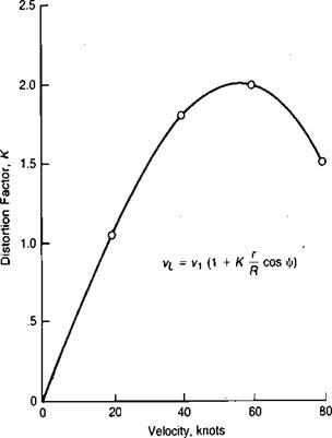
FIGURE 3.5 Induced Velocity Distortion Factor at Low Airspeeds |
Source: Ruddell, “Advancing Blade Concept (ABC) Development,” JAHS 22-1, 1977
The corresponding induced power is:
h – D™V – Г P’ind 550 l,100p AV
Note that, for a constant rotor thrust, the induced power decreases as forward speed increases. This is a consequence of the rotor handling more air per second and having to accelerate it downward less to achieve the same thrust.
The derivation so far has been based on an ideal rotor, analogous to an ideal wing with an elliptical lift distribution. The airplane aerodynamicist accounts for the fact that a wing seldom has an elliptical lift distribution by using an Oswald efficiency factor, e, in the denominator of the induced drag equation:
ind їїА. К.е
where e is less than unity. For a rotor, a corresponding rotor efficiency factor can be evaluated by comparing the distribution of circulation in the wake with an ideal
elliptical distribution. This was done in reference 3.7, in which the circulation distribution in the wake of an infinite-bladed rotor was computed from a blade element method assuming an uniform induced velocity distribution at the rotor. Figure 3.6 shows the computed distribution of circulation for a specific flight condition and the value of e that corresponds to this distribution. Figure 3.7 shows the results of the evaluation in rerms of e as a function of the angle of attack of the tip path plane for several values of tip speed ratio, Cr/’o, and twist. The angle of attack of the tip path plane for use in this type of analysis can be approximated by:
![]() D
D
aTPP = -57.3————–
 |
TPP G. W
computed, and the increments of induced drag due to these velocities are integrated to give the total rotor-induced drag. This type of analysis, of course, is more accurate but also more work. Reference 3.8 gives the results for only one point corresponding to a two-bladed UH-1 helicopter with —12° of twist at a tip speed ratio of.26, a Ct/g of 0.09, and a rotor angle of attack of about —9°. The value of e calculated by this method is 0.26 compared to 0.75 interpolated from Figure 3.7. Some, if not all, of the difference may be due to the difference in the number of blades used in the two analyses. Further calculations of this type should lead to a better understanding of the effects of different numbers of blades.
The equation for the induced power is:
or, alternatively:
Since most performance calculations are done with a blade element approach, the use of the rotor efficiency factor is limited. It does, however, provide some insight into what portion of the total power is induced power and how this portion is affected by flight conditions. It can also be used in the analysis of flight and wind tunnel test data, where it is desired to divide the total power into its various components.
The calculated induced power for the example helicopter using the efficiency factor of Figure 3.7 is shown in Figure 3.8 as a function of forward speed.
The rotors of a tandem rotor helicopter cannot be treated as two independent rotors since they aerodynamically interfere with each other. The effect is primarily one of the rear rotor operating in a "climb” condition, due to the downwash of the front rotor. The induced velocity at the rear rotor due to the front rotor can be estimated using theoretical charts such as those presented in reference 3-9. Figure 3.9 summarizes the results for several relative rotor positions as the ratio of induced velocity at the rear rotor to the induced velocity at the front rotor, kv/vx as a function of the wake skew angle, x, where:
V
x — tan —
 |
(л – = 0 in hover and approaches 90° in high-speed flight.) The increase in power is:
where T is the thrust of one rotor.
For side-by-side configurations, the streamtube has the same diameter as the total span of the rotors, and thus the induced velocity corresponding to a given thrust is less than on a single rotor. The same consideration applies to a tandem rotor helicopter in sidewards flight, and, as a matter of fact, tandems are flown sideways at low speeds when maximum takeoff performance is desired.
The power required to overcome the drag of all the nonrotor components is known as the parasite power, h. p.A
![]()
 |
550
The parasite drag could be expressed as a function of a drag coefficient as it is in airplanes:
Dp = CDqS
but in the case of a helicopter without a wing, the assignment of a reference area, S, is not a straightforward procedure. For instance, using the rotor disc area as a
![]()
|
|||
|
|||
|
|||
|
|||
|
|
||
|
|||
|
|||
|
|||
|
|||
|
|||
|
Equations for the induced velocities in hover were derived using the momentum method. A variation of the same method applies to forward flight and starts with the same equation:
T = m/sec x Av
In order to define the mass flow and the change in velocity, it is helpful to go back to the aerodynamics of a wing for an analogy. When a wing generates lift, at least in theory, it affects all the air, both near and far. Of course, the air adjacent to the
wing is affected the most, whereas at large distances from the wing the effect is negligible. It may be shown that for an ideal wing with an elliptical lift distribution, the downward acceleration of the total mass of air is mathematically equivalent to uniformly accelerating only the mass of air in a round stream tube whose diameter is equal to the wing span. This purely mathematical coincidence should not be given a physical connotation. For the wing shown in Figure 3.2, the momentum equation may be written:
|
|
|
|
|
|
 |
For most forward flight conditions, it may be assumed that vl is small compared with V, so that:
, aTPP will always be assumed to be small enough that: cos сц-рр = 1.
Using this definition, another alternative form for the induced velocity equation is:
SIR CT
p =————-
H 2
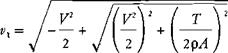
These equations apply to conditions where the forward velocity is relatively large with respect to the induced velocity. It is sometimes necessary to make calculations at low speeds, where this assumption is not valid. For these cases, the momentum equation is:
T=f>Ay/V2 + vl 2v, Solving this without making any assumptions gives:
|
|
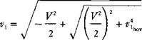
or:
|
|
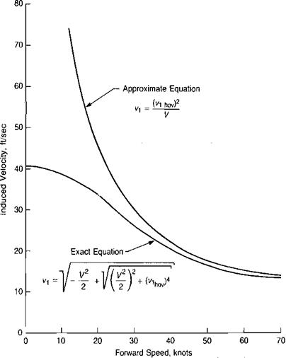
A comparison of the results of using this equation and the simpler one derived earlier is shown in Figure 3.3, where vx in ft/sec is plotted against forward speed in knots for the example helicopter. It may be seen that for the example helicopter, the two equations give essentially the same results above about 30 knots.
The simple equation for induced velocity derived here is known as the constant momentum induced velocity. A more realistic view sees the induced velocity as the result of a very complex vorticity pattern, consisting of trailing, shed, and bound vortex elements associated with the lift and the change of lift on each blade element. This complexity is of great importance when studying blade loads and helicopter vibration, but it has been found that for most performance calculations the use of the constant momentum value—which represents the average of the complex velocity field—gives reasonably accurate results. There are, however, two helicopter trim problems that require modifications to the simple theory. The first of these is the calculation of the effects of the rotor wake impinging on a horizontal stabilizer in low-speed forward flight. In hover, the average dynamic pressure in the fully developed wake is equal to the disc loading. Experience has shown, however, that local dynamic pressures in the wake in hover and forward flight may be significantly higher than this. Some feeling for this may be obtained by studying the plots of the wake dynamic pressure below a hovering rotor, which were shown in Figure 1.19 of Chapter 1. Test results reported in reference 3.1 show that the download pressure to which a horizontal stabilizer may be subjected in low-speed flight can be as much as three times the main rotor disc loading. Assuming a drag coefficient of 2 for the stabilizer in this condition gives a dynamic
|
FIGURE 3.3 Induced Velocities in Low-Speed Flight for Example Helicopter |
pfessure in the wake of 1.5 times the disc loading. This can be the source of disconcerting trim shifts in transition flight.
Another analysis problem that will be examined in detail later is that of calculating the lateral blade flapping in forward flight. For this, it has been found necessary to represent the local induced velocity at the disc as:
v=vA 1 + К — cos w I * /
where j/ is the blade azimuth position, being zero over the tail. This equation defines an induced velocity distribution that is small at the leading edge of the disc and large at the trailing edge, as shown in Figure 3.4. Smoke studies of the induced velocities around wind tunnel models of rotors in forward flight reported in references 3.2 and 3.3 show that the average velocity distribution does indeed have
 |
this general pattern and, furthermore, that the induced flow at the leading edge of the disc is essentially zero. This observation leads to assigning the distortion factor, К, a value of unity, so that:
This applies to relatively high speeds—say above 100 knots—but at low speeds, the distortion may be somewhat higher. This is shown in Figure 3.5, taken from reference 3.4, which reports on flight tests and wind tunnel experience on the very rigid rotor Sikorsky Advancing Blade Concept helicopter. From the cyclic pitch required to trim, the distortion factor in the induced velocity equation could be determined. The figure indicates that while a value of unity may be good for high speeds, in the transition region it may be as high as 2.
Several alternative forms of this equation are discussed in reference 3.5, a study of the surprisingly large lateral flapping that occurs at low speeds.. A more rigorous derivation of the induced velocity distribution using vortex theory is given in reference 3.6.
MOMENTUM AND ENERGY CONSIDERATIONS
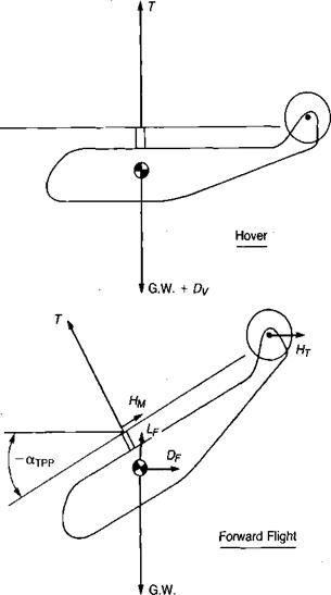
Just as in hover and vertical flight, there are two basic methods for analyzing the characteristics of a rotor in forward flight: the momentum, or energy, method; and the blade element method. The blade element method is necessary for accurate performance estimation and for establishing the limits of rotor performance, but the momentum method provides a rapid means of obtaining a first estimate of the performance as well as a valuable insight into the physics of the system. The balance of forces that governs the helicopter in forward flight is shown in Figure 3.1. The rotor thrust vector must balance not only the gross weight, as it does in hover, but also the horizontal drag of the rotor blades and the lift and drag of the fuselage, hub, landing gear, and other necessary—but draggy—items by which helicopters achieve their role as useful vehicles. The drag of the rotor blades is known as the rotor horizontal force, or H-force, and all other drag items are classified as parasite drag.
|
FIGURE 3.1 Balance of Forces on Helicopter |
The instantaneous thrust and power associated with a vertical flight condition is affected by the rate of change of collective pitch. This is of some significance in its effect on performance during jump take-offs and in landing flares from vertical autorotation. It is of even more significance in its effect on the design of a tail rotor drive system.
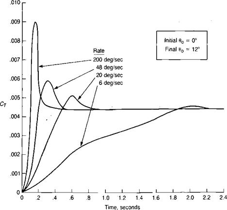
The phenomenon may be illustrated by visualizing a rotor with untwisted blades on a whirl tower at full rotor speed and flat pitch. If the collective pitch is suddenly increased to 10°, the angle of attack of each blade element will instantaneously be 10° and then will decrease as the equilibrium-induced flow pattern is established. Figure 2.15 taken from reference 2.15, shows the measured thrust coefficient of a 33-foot-diameter rotor on a whirl tower for several rates of collective pitch inputs. It may be seen that for very rapid increases, a transient thrust overshoot to twice the final steady value is possible. Not only does the thrust have an overshoot but the torque may also; especially if the transient angles of attack produce stall.
For the main rotor, the transient increase in torque required may exceed that available from the engine and the rotor will slow down, the extra power required being produced by the loss in rotational kinetic energy. Such a decrease is usually safe unless the rotor slows to a point where it can no longer produce the required
|
FIGURE 2.15 Effect of Rapid Pitch Change on Rotor Thrust |
Source: Carpenter & Fridovich, “Effect of a Rapid Blade-Pitch Increase on the Thrust and Induced-Velocity Response of a Full-Scale Helicopter Rotor,” NACA TN 3044, 1953.
thrust. The situation is different for a tail rotor, however. The transient increase in torque is small compared with the total inertia of the rotating system so that little or no slowing takes place and the tail rotor simply demands whatever torque is required from its drive system. This torque may be several times the maximum steady torque which might reasonably be used in the design of the tail rotor drive system. The most critical flight maneuver is stopping a turn over a spot in the torque direction (analogous to vertical descent of the main rotor) with full opposite pedal. For this case, the instantaneous change in angle of attack may be as much as 30° which will insure fully stalled blades and a correspondingly high torque requirement compared with normal flight. In lieu of designing the tail rotor drive system to take this abnormally high torque, the current practice is to design for some more moderate loading—for example, twice the maximum hover torque—and then to ask the pilots to refrain from extreme turn-reversal maneuvers. In some cases, helicopters have been equipped with dampers on the rudder pedals to make it difficult for the pilot to apply sudden pitch changes.
EXAMPLE HELICOPTER CALCULATIONS
![]()
![]() Power required in vertical climb Rate of descent for maximum roughness Rate of descent in vertical autorotation
Power required in vertical climb Rate of descent for maximum roughness Rate of descent in vertical autorotation
HOW TO’s
The following items can be evaluated by the methods in this chapter.
Collective pitch in vertical autorotation Extra power required for vertical climb Induced velocity in climb Induced velocity in windmill brake state Induced velocity distribution in vertical climb Region of power settling
Speed for maximum roughness in vortex ring state Rotor thrust damping Rate of descent in vertical autorotation

Even though vertical autorotation occurs in the vortex ring state, a first approximation procedure for calculating the rate of descent may be derived from a combination of blade element and momentum concepts. Setting the torque equation for the ideally twisted rotor to zero gives:
![]()
|
|
||
![]()
|
|
|
|
Sideward Speed, knots
Source: Prouty, “Development of the Empennage Configuration of the YAH-64 Advanced Attack Helicopter," USAAVRADCOM TR-82-D-22, 1983.
where from the hovering derivation:
(0r — фг) = CT ——
The inflow angle at the tip, фт, is:
 |
Source: Castles & Gray, “Empirical Relation between Induced Velocity, Thrust, and Rate of Descent of a Helicopter Rotor as Determined by Wind-Tunnel Tests of Four Model Rotors,” NACA TN 2474, 1951.
This result is so typical that a rule of thumb is that the rate of descent in vertical autorotation is twice the hover-induced velocity. This is also borne out by an examination of Figure 2.8. Figure 2.13 shows that an untwisted rotor is better than a twisted one for vertical autorotation in that a lower rate of descent is required.
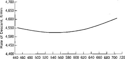
The rate of descent is a function of rotor speed; the minimum ocurring at the rotor speed that corresponds to the maximum c,/2/q. Figure 2.14 shows the calculated rate of descent of the example helicopter as a function of rotor speed. The minimum rate of descent occurs at a tip speed of about 550 ft/sec. Although this represents a theoretical optimum, it is not a practical condition since the rotor is on the verge of blade stall, which could be triggered by small changes in flight conditions, and because of the relatively low value of kinetic energy stored in the rotor for use in the landing flare. It is more likely that the pilot would try to hold
|
|
|
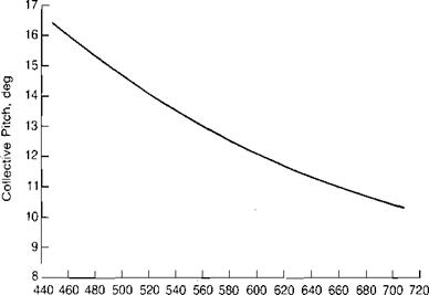
the normal power-on tip speed or even a value slightly higher. The collective pitch required as a function of tip speed can be estimated by combining equations already derived.
3 3
0O = — 0T –0, 0 2 ^Idcal twist ^ 1
For these calculations, no power losses due to the transmission, accessories, or tail rotor have been considered. For actual cases where the rotor must supply the extra power, Ah. p., the equation for the velocities becomes:
|
1 ( 4,400Ah. p. |
|
|
P Ab^ClRycd_ |
|
For the example helicopter, it is estimated that the rotor must develop 40 hp during vertical autorotation. This will increase the value of (VD — by 11%, but the rate of descent will increase by only 1.5%. It is of some interest to note that the rate of descent of a parachute is given by the equation:
For a parachute with the same disc loading as the example helicopter and a drag coefficient of 1.2, the rate of descent is 4,260 ft/min—approximately the same as the helicopter. This comparison adds validity to the observation that the rate of descent of the helicopter in autorotation is approximately twice the hover – induced velocity. (A parachute with a drag coefficient of 1.0 would be an exact analogy of the helicopter in this condition.)
Flight in the vortex ring state is characterized by very unstable flow conditions, which produce vibration and erratic thrust variations. Flight test experience on a small tandem rotor helicopter reported in reference 2.3 showed that the characteristic vibration began at a rate of descent equal to about 23% of the hover – induced velocity and persisted until the rate of descent exceeded 125% of the hover-induced velocity.
For the example helicopter, these boundaries would cover the region between 400 and 2,900 ft/min rate of descent. The results also showed that for the test helicopter, forward speeds above about 10 knots were sufficient to avoid vortex ring vibration at all rates of descent. Similar tests on a larger single-rotor helicopter reported in reference 2.4 showed that a forward speed of 25 knots was enough to avoid the vibration. Thus, in flight, it is relatively easy to get out of the vortex ring state by flying with a small amount of forward speed. As a matter of fact, it is a fairly difficult piloting task to stay in the vortex ring state for any length of time.
![]()
|
|
|
|
|
|
|
|
|
|
|
![]()
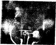
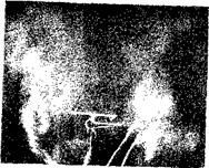
Source: Drees & Hendal, "Airflow Patterns in the Neighborhood of Helicopter Rotors,” Aircraft
Engineering, Vol. 23, April, 1951. Photos courtesy of MLR.
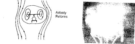
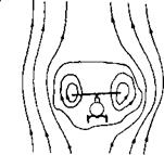
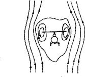
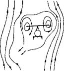
The instability of the vortex ring flow studied with smoke going through a model rotor in a wind tunnel was reported in reference 2.5. Two observations in that report are of interest in visualizing the flow. The first speculates about an effective airbody within which air is circulated by the rotor, as shown in Figure 2.5. The airbody is originally roughly spherical; but, as the rotor pumps energy into it, it lengthens downward until it bursts like a bubble, permitting the accumulated energy to dissipate into the surrounding upward-moving air. The airbody then returns to its original shape and starts the cycle again. The fluctuating airflow, of course, makes the thrust and/or rate of descent also fluctuate. The other observation based on a study of the smoke pictures (especially vivid in the motion pictures made during this study) is that the airflow fluctuations are not symmetrical around the rotor. Figure 2.5 shows several frames from the smoke movies during a steady vortex ring condition. The vortex can be seen to be formed first on one side and then on the other in a completely random fashion. Thus not only does the rotor thrust fluctuate, but so also does the flapping as the rotor responds to the changing inflow patterns.
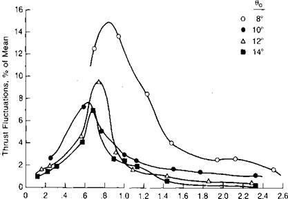
The magnitude of the vortex ring flow fluctuations as measured on a model rotor in a wind tunnel are reported in reference 2.6 and are shown in Figure 2.6. The region of roughness is about the same as that found in flight test. A theoretical study of the vortex ring state presented in reference 2.7 concludes that the maximum wake instability should occur for the condition in which the tip vortices stay in the plane of the rotor. Reference 2.7 shows by a momentum
|
|
V<> v’ ho»
FIGURE 2.6 Thrust Fluctuations in Vertical Descent
Source: Azuma & Obata, "Induced Flow Variation of the Helicopter Rotor Operating in the Vortex Ring State,” Jour, of Aircraft, July-August, 1968.
m
analysis that this condition exists when the rate of descent is equal to 0.707 times the induced velocity in hover. This conclusion is verified by Figure 2.6. A further study of vortex ring theory is presented in reference 2.8.
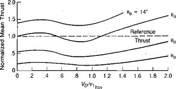
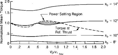
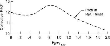
The experimental data of reference 2.6 also illustrates the phenomenon known to pilots as power settlings where more power is required to descend than to hover. Figure 2.7 shows normalized thrust and torque values as a function of the vertical descent velocity ratio. A reference thrust level has been selected— corresponding to hover at 12° of collective pitch—and the required collective
|
|
|
|
|
FIGURE 2.7 Effect of Rate of Descent on Rotor Conditions |
Source: Azuma & Obata, “Induced Flow Variation of the Helicopter Rotor Operating in the Vortex Ring State,” Jour, of Aircraft, July-August, 1968.
pitch and torque as a function of rate of descent have been found by crossplotting. It may be seen that both the required pitch and torque first decrease, as would be expected, and then increase in the region of maximum flow fluctuation before decreasing again as the rotor approaches autorotation. The power-settling condition is of practical importance if during a vertical takeoff of a multiengined helicopter, one engine fails and the pilot attempts to return vertically to the takeoff point. If during this return the pilot enters the power-settling region, the power required from the remaining engines—or the final impact velocity—will be higher than would be estimated from simple transfer-of-energy equations. This region also roughly corresponds to the region of negative thrust damping. A detailed analysis of vertical and near-vertical descent will be found in reference
2.9.
|
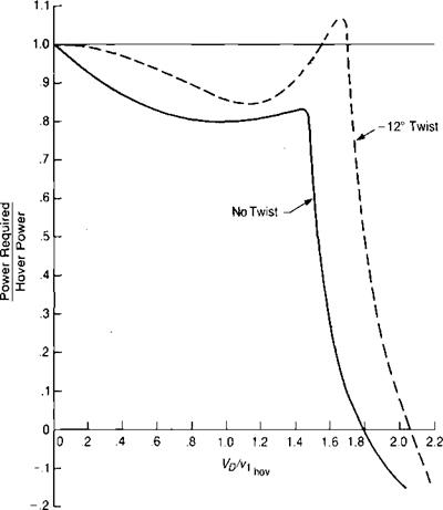
FIGURE 2.8 Effect of Twist on Power Required in Vertical Descen |
Source: Castles & Gray, “Empirical Relation between Induced Velocity, Thrust, and Rate c Descent of a Helicopter Rotor as Determined by Wind-Tunnel Tests of Four Model Rotors,” NAC TN 2474, 1951.
An as yet unexplained mystery is indicated by Figure 2.8, which presents an analysis of wind tunnel data reported in reference 2.10 for two model rotors, which were identical’ except for blade twist. The rotor with the twisted blades demonstrated a definite power-settling regime, whereas the rotor with untwisted blades did not. In addition, the authors comment: "Also, the fluctuations in the forces and moments on the rotor with twisted blades were very much larger at the higher rates of descent than for the rotors with untwisted blades.”

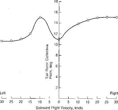
Vertical descent is not the only flight condition in which the vortex ring state is of importance. A tail rotor may be operated in the vortex ring state during sideward flight or during a hover turn over a spot. Figure 2.9 shows the tail rotor collective pitch as a function of sideward velocity for the UH-1 as reported in reference 2.11. The "lump” is attributed to the vortex ring state. In the region of neutral and negative slope to the left of hover, pilots find it very difficult to hold a steady
|
FIGURE 2.9 Tail Rotor Pitch Required in Sideward Flight |
Source: Lehman, “Model Studies of Helicopter Tail Rotor Flow Patterns In and Out of Ground Effect,” USAAVLABS TR 71-12, 1971.
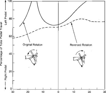
heading. Hover turns that put the tail rotor in this condition, create a situation that pilots call "falling into a hole.” The basic cause of this is best illustrated by the curves in the top portion of Figure 2.7. The curves are unstable between velocity ratios of 0.4 and 0.8, and any increase in the turn rate will lower the tail rotor thrust, thus increasing the rate even further. The hover-induced velocity for the UH-1 tail rotor is about 48 ft/sec. The maximum vortex ring effect would be expected to occur at 70% of this value or at about 20 knots. The fact that it occurs at a lower speed appears to be a result of the main rotor wake interacting with the tail rotor. Figure 2.10, taken from reference 2.12, shows a dramatic difference in pedal position in sideward flight resulting from a change in the direction of tail rotor rotation for the Lockheed AH-56A. Rotation with the bottom blade going aft apparently entrains the tip vortex of the main rotor, causing a premature vortex ring condition at the tail rotor. Rotation in the opposite direction seemed
|
Left Sideward Flight Right Sideward Flight Velocity, knots FIGURE 2.10 Typical Pedal Requirements for AH-56A in Right and Left Sideward Flight |
Source: Wiesnerand Kohler, “Tail Rotor Design Guide,” USAAMRDLTR 73-99,1973.
to cause an indefinite delay in the vortex ring condition resulting from a favorable interference of the main rotor tip vortex.
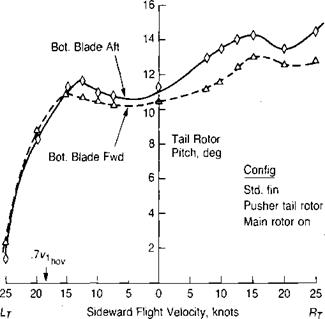
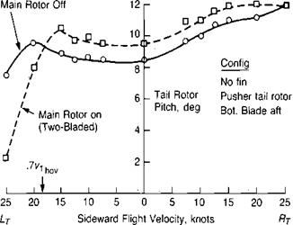
Experimental evidence of this interference is given in reference 2.13. Figure 2.11, based on that report, shows the pitch of the tail rotor required to balance main rotor torque as a function of sideward speed for four different model configurations. The top portion shows the effect of the presence of the main rotor and the lower portion shows the effect of tail rotor direction of rotation in the presence of the main rotor. The evidence of premature vortex ring conditions is not as dramatic as in the preceding two figures, but it is there.
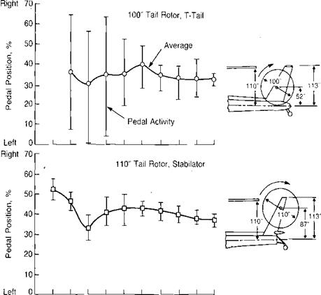
Another study of left sideward flight motivated by some less-than – satisfactory sideward-flight characteristics discovered during the initial development flying on the Hughes AH-64 is reported in reference 2.14. Figure 2.12 shows the pedal activity required to hold heading in left sideward flight with two different tail configurations: a T-tail with a 100-inch diameter tail rotor and a stabilator with a 110-inch diameter tail rotor. The improvement observed with the second configuration was also present even when flown with the smaller tail rotor. Thus the beneficial change appears to be due to raising the tail rotor, which apparently made it less susceptible to effects from the main rotor tip vortices. Two further observations from this program are worth mentioning. The same test pilots who were investigating the unsatisfactory left-sideward-flight characteristics of the AH-64 with the T-tail found that a Huey Cobra that was available as a chase aircraft had no trouble in the same flight condition even with its stability augmentation system turned off! The Cobra tail rotor blades are untwisted, whereas those on the AH-64 have —8° of twist. The differences seem to correlate with the wind tunnel experience quoted during the discussion of Figure 2.8.
The other observation is that on the AH-64, pure left sideward flight was not the most critical condition. Instead, the unsteadiness was worse, with the aircraft flying about 20° off of pure left with the tail rotor leading the main rotor. Why this should be more critical than with the tail rotor following the main rotor is not known.