Category Management and Minimisation of Uncertainties and Errors in Numerical Aerodynamics

Numerical Study of the Influence of Geometrical Uncertainties (Testcase SFB-401)

The influence of geometrical uncertainties on flow parameters is investigated con­sidering the 3d testcase SFB-401 (Navier-Stokes flow). A detailed overview and in­troduction to uncertainty quantification methods can be found in [42], [35], [24]. We will concentrate in the following on a Polynomial Chaos approach which expands the solution nonlinearly depending on the random variable з or random vector re­spectively, in a series of orthogonal polynomials with respect to the distribution of the random input vector

f (У,P, s(O) = X aі(У’P) ■ ф(s(Z)) (76)

i=1

with Фі orthogonal polynomials, ai(y, p) deterministic coefficient functions. For a detailed discussion of the method, we refer to [41]. The basic idea of Polynomial Chaos representing the stochastic output of a differential equation with random input data is to reformulate the SDE replacing the solution and the right hand side of the PDE by a Polynomial Chaos expansion. Given a stochastic differential equation of the form

L(x, t,Z;u)= g(x, t, Z), X e G, t Є [0, T], Z e a (77)

where u = u(x, t, Z) is the solution and g(x, t, Z) is the right hand side. The operator L can be nonlinear and appropriate initial and boundary conditions are assumed. Replacing pointwise the solution u = u(x, t, Z) of equation (77) by the Polynomial Chaos expansion leads to

M

u(x, t, Z) = X uk(x, t)Фк(s(Z)) (78)

k=1

where uk(x, t) are the deterministic Polynomial Chaos coefficients which need to be determined. Furthermore, the right hand side g(x, t, Z) will be also expanded by a Polynomial Chaos expansion

M

Подпись: (79)Подпись:g(xt, Z) = X gk(x>t)фк(3(Z))

k=1

and the deterministic coefficients are given by

< g(x, t, ■)ф >

< ф2к >

In the literature, two different classes of methods determining the unknown coeffi­cients uk(x, t) are proposed: non-intrusive and intrusive Polynomial Chaos. As the intrusive methods require a modification of the existing code solving the determin­istic PDE (if the Operator L is nonlinear), this drawback of the method force us
Numerical Study of the Influence of Geometrical Uncertainties (Testcase SFB-401)

to consider non-intrusive Polynomial Chaos methods which allow to use the flow solver as a black-box. The unknown coefficients are given by

whereas the integral of equation (82) is approximated by a sparse grid approach.
Подпись: Fig. 27 Perturbed region of the SFB-401 profile

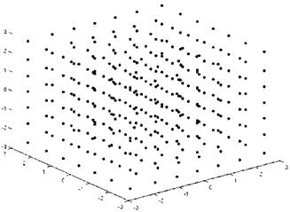
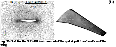
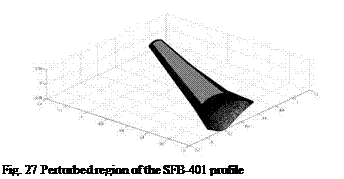
In the 3d testcase, the space is discretized by 2506637 grid points, where the surface is described by 80903 points. The grid generated with Centaur con­sists of 1636589 tetraeders, 4363281 prisms and 170706 surfacetriangles, 5427 surfacequadrilaterals, see Fig. 26. The geometrical uncertainties are assumed to oc­cur on the upper side of the wing, the perturbed region is depicted in Fig. 27. The perturbations are modeled as a Gaussian random field with the following second order statistics
Подпись: Projection in 2d of the SFB-401 profile

Fig. 28

E (y(x, Z)) = 0 Vx Є Г (83)

Cov(x, y) = (0.0016)2 – exp Vx, y Є Г. (84)

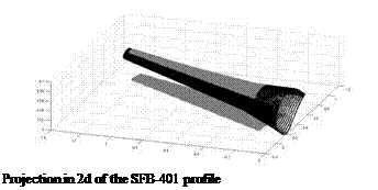
In order to take the curvature of the wing into account computing the norm in (84), the selected area is transformed into 2d approximating the distance by a polygon path on the surface. The projection is depicted in Fig. 28 Due to the problem size, an iterative eigensolver BLOPEX (cf. [28]) is used in order to solve the eigenvalue problem arising from the Karhunen-Loeve expansion. The resulting eigenvalue dis­tribution of the first 50 eigenvalues is shown in Fig. 29.

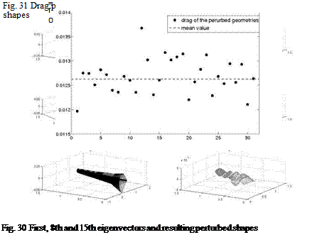
We consider the first 15 eigenvalues and eigenvectors to represent the random field, as an example the first, 8th and 15th eigenvectors and resulting perturbed shapes are depicted in Fig. 30.

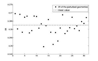
In order to approximate statistics of the flow solution depending on the con­sidered perturbations, the drag, the lift and the pressure coefficient cp are expanded into the first 16 multidimensional Hermite polynomials. In the next two figures (Fig. 31, Fig. 32), the drag and the lift of each perturbed shape and the corresponding

x 10 1

0 5 10 15 20 25 30 35 4 0 45 50
Numerical Study of the Influence of Geometrical Uncertainties (Testcase SFB-401)
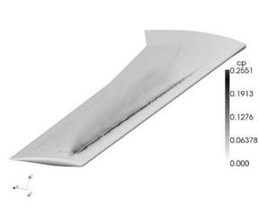
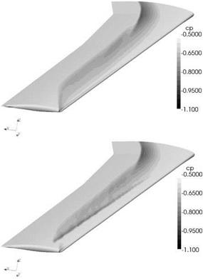
mean values are illustrated. As Fig. 31 indicates, the geometry uncertainties have a large impact on the target functional. The standard deviation from the mean value is equal to 1.65 drag counts, and the mean value is 6.55 drag counts higher than the nominal, unperturbed geometry. The comparison between the Cp distribution of the unperturbed geometry and the Cp distribution of the mean value shows that an

Numerical Study of the Influence of Geometrical Uncertainties (Testcase SFB-401)

Fig. 32 Lift performance and mean value of the perturbed 3d shapes

additional shock on the upper side of the shape occurs due to the uncertainties in the geometry (cf. Fig. 34). Fig. 33 emphasizes the influence of the perturbations showing the variance of the cp distribution.

8 Conclusions

Robust design is an important task to make aerodynamic shape optimization relev­ant for practical use. It is also highly challenging because the resulting optimiza-

Numerical Study of the Influence of Geometrical Uncertainties (Testcase SFB-401)

Numerical Study of the Influence of Geometrical Uncertainties (Testcase SFB-401)

Fig. 34 Comparison between the cp distribution of the unperturbed geometry (above) and the cp distribution of the mean value (below)

tion tasks become much more complex than in the usual single set-point case. The comparison of the two robust optimization formulations shows that the discretized semi-infinite formulation seems to be of advantage in a numerical test case close to a real configuration. In the case of the geometric uncertainty, the approximation of the random field describing the perturbations of the geometry leads to a very high di­mensional optimization task. The dimension of the probability space was efficiently reduced by a goal-oriented choice of the Karhunen-Loeve basis. Furthermore, ad­aptive Sparse Grid techniques and one-shot methods have been successfully gener­alized to the semi-infinite formulation of the shape optimization problem in order to reduce the amount of computational effort in the resulting robust optimization. The numerical results show that even small deviations from the planned geometry have

a significant effect on the drag and lift coefficient, so that geometry uncertainties have to be taken into account in the aerodynamic design optimization problem to ensure a robust solution. The introduced methods can significantly reduce the costs of the robust optimization, so that robust design becomes numerically tractable in the aerodynamical framework.

[1] See http://aaac. larc. nasa. gov/tsab/cfdlarc/aiaa-dpw

[2]-2 10-1 10° 101 102

reduced frequency, ©

Fig. 16 Fourier-transformed fluctuations of lift coefficient Cl and corresponding fluctuations over time for an LES simulation

Volker Schulz • Claudia Schillings

FB IV Department of Mathematics, University of Trier, Universitatsring 15,

54296 Trier, Germany

e-mail: {volker. schulz, claudia. schillings}@uni-trier. de

[4] MEGADESIGN Aerodynamic simulation and optimization in aircraft design, German na­tional project funded by the German Federal Ministry of Economics and Labour (BMWA).

B. Eisfeld et al. (Eds.): Management & Minimisation of Uncert. & Errors, NNFM 122, pp. 297-338. DOI: 10.1007/978-3-642-36185-2_13 © Springer-Verlag Berlin Heidelberg 2013

Navier-Stokes Flow

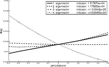
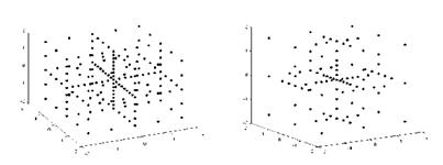
As in the Euler case, we investigate the influence of the individual eigenvector of the Karhunen-Loeve expansion on the target functional depicted in Fig. 18 Since the third eigenvector has no impact on the target functional, the mean value is ap­proximated using the first, second and fourth basis vector (cf. (75)). If the same error tolerance 3 • 10~4 as in the previous testcase is required, a full grid of 4913 grid points based on multilinear ansatzfunctions has to be used in order to compute the objective function. A reduction factor of 28 can be achieved by a sparse grid approach which is further improved by a local refinement strategy. The resulting adaptive grid consists of 99 grid points.

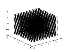
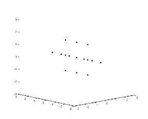
Since the computational effort in the Navier-Stokes case is much higher than in the Euler testcase, the number of grid points need to be further reduced in order to make a robust optimization possible. The use of Gaufi-Hermite quadrature formulas results in the same full grid and sparse grid shown in Fig. 13 and Fig. 14 as in the Euler testcase fullfilling the error tolerance 3 • 10~4. The dimension adaptive approach leads to the following grid 21.

Navier-Stokes Flow

Navier-Stokes Flow

Fig. 19 Full tensor grid with 4913 grid points

Navier-Stokes Flow

Fig. 20 Sparse grid with 177 grid points and locally refined sparse grid with 99 grid points

Navier-Stokes Flow

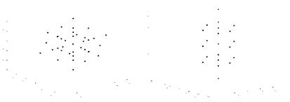
Fig. 21 Dimension adaptive sparse grid with 15 grid points (Navier-Stokes flow)

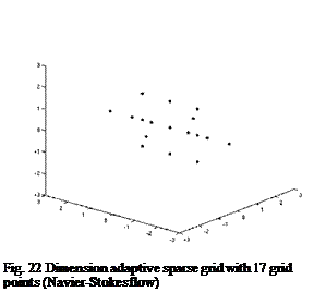
Подпись: Fig. 22 Dimension adaptive sparse grid with 17 grid points (Navier-Stokes flow)
The linearity of the drag depending on the first eigenvector (cf. 18) is recognized by the dimension adaptive algorithm, so that this dimension is not further refined. Since the linear behaviour might change during the optimization, we add two points ensuring that the first eigenvector is taken into account during the optimization, see Fig. 22. Fig. 23 and 24 illustrate the drag and lift performance of the 17 perturbed geometries of the single setpoint and robust optimization.

Navier-Stokes Flow Подпись: 10 Подпись: 14 Подпись: 16

The mean value of the drag in the robust case is a little bit higher than the mean value of the single setpoint optimization (5 drag counts) which can be attributed to the lift constraints. The robust optimization is feasible over the whole range of

Navier-Stokes Flow

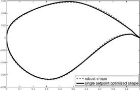
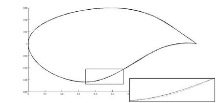
perturbations as required, whereas the single setpoint optimization cannot reach the target lift in more than 60 % of the realizations. Hence, we can state that the semi­infinite optimizations leads to a better lift to drag ratio as in the Euler case. The resulting shapes are depicted in Fig. 25. The difference between the robust shape and the single setpoint optimized shape is smaller than in the Euler case, indicating that the profile is more sensitive to changes of the shape.

Euler Flow

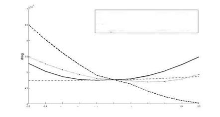
As Fig. 10 shows, the third eigenvector has no impact on the objective function, hence it can be rejected from the Karhunen-Loeve basis and the dimension of the integral is reduced. This behaviour is also reflected by the introduced indicator. Consequently, the mean value is given by

e(/ (y, P, yreduced (x, Z))) =

—— 1. eigenvector

indicator:

2.255806Є-04

—– 2. eigenvector

indicator:

-1.421137e-03

— 3. eigenvector

indicator:

7.722186Є-06

■■"•■■■4. eigenvector

indicator:

-4.745173Є-04

Euler Flow

-0.3 -0.2 -0.1 0 0.1 0.2 0.3

perturbations

Fig. 10 Drag performance of the first four eigenvectors on the target functional

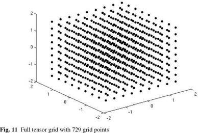
If one approximate the expected value (75) using a full tensor grid interpolation (40), 729 grid points will be needed to reach the error tolerance of 3 • 10_4. The resulting full grid is shown in Fig. 11. Since we want to compare the efficiency of the different introduced methods, we have chosen multilinear hierarchical basis function as ansatzfunctions for the sparse and full tensor grid. The sparse grid method can reduce the computational effort by a factor of 10 maintaining the same approximation quality. The corresponding grid is depicted in Fig. 12. As Fig. 12

Euler Flow

Euler Flow

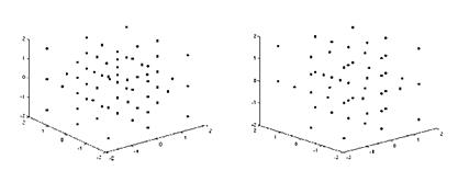
Fig. 12 Sparse grid with 69 grid points and locally refined sparse grid with 52 grid points

shows, the number of grid points can again be reduced from 69 grid points to 52 grid points, i. e. a reduction of 17 flow simulations in each iteration is reached us­ing a local refinement strategy. Since the optimization requires the evaluation of the mean value in each iteration, this reduction by factor 15 compared with the full grid takes place in each step of the optimization algorithm and hence significantly speed up the whole algorithm. The construction of the adaptive sparse grid although needs some additional function evaluations in order to compute the adaptivity indicator, but this amount of computational effort occurs outside the optimization loop, i. e. these costs are negligible.

Beside the local refinement strategy, a dimension adaptive sparse grid was in­troduced in section 5.1. The main advantage of this approach lies in the possibility to choose the underlying quadrature formulas problem dependent. As discussed be­fore, Gaufi-Hermite formulas are used. Due to the higher accuracy of Gaufi-Hermite

Euler Flow

Fig. 13 Full tensor grid with 343 grid points

Euler Flow

Fig. 14 Sparse grid with 37 grid points and dimension adaptive sparse grid with 21 grid points


quadrature formulas, an error tolerance of 10~5 is required. An usual sparse grid can reduce the number of grid points from 343 to 37, again almost a factor of 10. The dimension adaptive strategy results in a grid with 21 points (cf. Fig. 14). The comparison of the two refinement strategies shows that the use of problem dependent quadrature formulas can significantly reduce the size of the grid and in­crease the approximation quality at the same time. Hence, the objective function in the semi-infinite formulation is approximated by the dimension adaptive grid with 21 grid points. the next two Fig. 15,16 compare the results of the robust optimization and of the single setpoint optimization, i. e. without considering any uncertainties

Подпись: 14 16 18 20 22‘ 0 2 4 6 8 10 12

Подпись: * single setpoint optimization * robust optimization target lift
Euler Flow
Подпись: 20 Подпись: 22
Подпись: 4 Подпись: 6 Подпись: 8

Fig. 16 Lift performance of the 21 perturbed geometries

Euler Flow

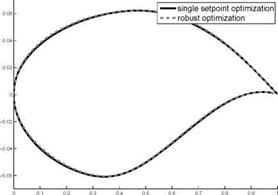
The drag and lift performance is plotted against the 21 perturbed geometries and the dashed line in Fig. 15 indicates the mean value of the drag. The robust optim­ization improves the mean value of the target functional and also leads at the same time to a better lift performance over the whole range of perturbations, whereas the single setpoint optimization is infeasible in more than the half of the considered grid points. Summing it all up, it can be said that the robust optimization leads to a better lift to drag ratio than the single setpoint optimization and the resulting profile is more robust against small perturbations of the shape itself. Last, we will compare the different resulting shape in Fig. 17.

Although we have assumed only small perturbations of the shape itself (cf. Fig. 7), the difference between the robust shape and the single setpoint is well recognizable.

Numerical Results Considering Geometrical Uncertainties (Testcase RAE2822)

In this section, we present the numerical results of robust optimization under shape uncertainties of a RAE2822 profile in Euler and Navier-Stokes flow. Since the robust optimization problem is solved within a one-shot framework, we use the flow solver TAU provided by DLR which allows the computation of gradients by the adjoint approach in the Euler and Navier-Stokes case. The TAU Code is a CFD software package for the prediction of viscous and inviscid flows about complex geometries from the low subsonic to the hypersonic flow regime employing hybrid unstructured grids. In the Euler case, the profile is described by 129 surface grid points and in the Navier-Stokes case, by 192 surface grid points. Again, the airfoil is parametrized by 21 Hicks-Henne functions. The geometry uncertainties are characterized by a Gaussian random field and the following second order statistics

E(у(х, Z)) = 0 Ух є Г (72)

Cov(x, y) = (0.005)2 • exp (-J^£) Vx, y є Г. (73)

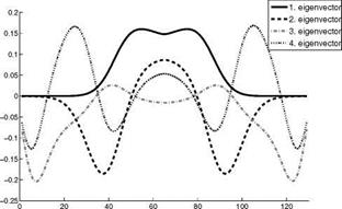
One realization of the random field and the resulting perturbed geometry is shown in Fig. 6 and Fig. 7. Representing the random field for the numerical treatment у in a finite number of independent random variables using the Karhunen-Loeve – Expansion, one has to solve the eigenvalue problem (9). In our two-dimensional testcase, the discretization of the profile leads to a matrix of size (129 x 129) and (192 x 192) in the Navier-Stokes case, so the eigenvalues and eigenvectors can be computed by common methods. The distribution of the eigenvalues of the given ran­dom field (72-73) is shown in the next Fig. 8. As stated before, the eigenvalues ex­ponentially converge towards 0. For the first numerical results, we have considered only the first four eigenvalues and eigenvectors to represent the random field у of

Numerical Results Considering Geometrical Uncertainties (Testcase RAE2822)

Numerical Results Considering Geometrical Uncertainties (Testcase RAE2822)

Fig. 6 One realization of the random field perturbations on the upper side of the profile (above) and on the lower side (below)

Numerical Results Considering Geometrical Uncertainties (Testcase RAE2822)

Fig. 7 Resulting perturbed geometry compared with the original shape (dashed line)

perturbations. The corresponding eigenvectors are shown in Fig. 9 Using the trun­cated Karhunen-Loeve representation, the mean value of the drag is then computed by

The random variables Yi are uncorrelated and therefore independent, so one has to approximate a four-dimensional integral in the optimization problem. To further reduce the computational effort, we investigate the influence of the individual eigen­vectors in order to reject those eigenvectors from the reduced basis which have no impact on the target functional. Since the following results are problem dependent, we will now distinguish the Euler and Navier-Stokes case.

Numerical Results Considering Geometrical Uncertainties (Testcase RAE2822)

8


6


Numerical Results Considering Geometrical Uncertainties (Testcase RAE2822)

0


Numerical Results Considering Geometrical Uncertainties (Testcase RAE2822)

80


120


20


40


60


Fig. 8 Distribution of the eigenvalues of the given random field у

Numerical Results Considering Geometrical Uncertainties (Testcase RAE2822)


Numerical Results Considering Geometrical Uncertainties (Testcase RAE2822)

Fig. 9 First four eigenvectors of the given random field у

Numerical Results

The numerical results include a numerical comparison of the introduced robust for­mulations considering the optimization of a transonic RAE2822 profile under scalar­valued uncertainties. Further, the optimal aerodynamic shape under geometrical un­certainties is computed in a 2d Euler and Navier-Stokes testcase comparing the ad­aptive refinement strategies of sparse grids. The last section shows the influence of shape uncertainties on the quantities of interest in the 3d testcase SFB-401.

7.1 Numerical Comparison of the Introduced Robust Formulations

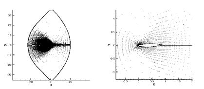
We investigate the shape optimization of a RAE2822 profile in transonic Euler flow, by the use of the CFD software FLOWer provided by DLR within a one-shot frame­work. The block-structured FLOWer code solves the three-dimensional compress­ible Reynolds-averaged Navier-Stokes equation in integral form and provides dif­ferent turbulence models. The equations are solved by a finite-volume method with second order upwind or central space discretization. The discrete equations are in­tegrated explicitly by multistage Runge-Kutta schemes, using local time stepping and multigrid acceleration. In our example, the space is discretized by a 133×33 grid, see Fig. 1. For parametrization, the airfoil is decomposed into thickness and camber distribution. Then, only the camber of the airfoil is parametrized by 21 Hicks-Henne functions and the thickness is not changed during the optimization process.

Numerical Results

Fig. 1 Grid for the RAE2822 airfoil: the total geometrical plane and zoom around the airfoil

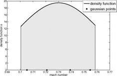
In this section, we consider the Mach number as an uncertain parameter. The Mach number is assumed to be in the range of [0.7,0.76]. Under the assumption of truncated normally distributed parameter, we obtain the density function shown below in the Fig. 2.

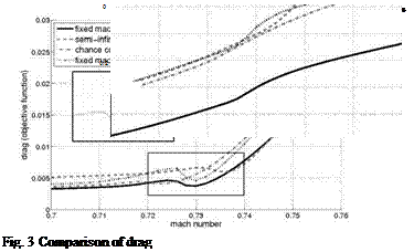
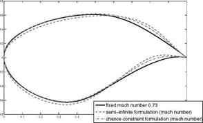
At first, we perform numerical comparisons between a single set-point prob­lem formulation at the setpoint s0 = 0.73Mach with the robust formulations in sections 3.2 and 3.3. In particular, we compare four formulations: (1) non-robust optimization at the Mach number 0.73 (fixed Mach number 0.73), (2) semi-infinite formulation of equations (26-28), (3) chance constraint formulation of equations (34, 35) and (4) non-robust optimization at the Mach number 0.73 (fixed Mach number 0.73) but maintaining feasibility over the whole range of perturbations.

The following figures show evaluations of the objective (drag), Fig. 3, in these cases as well as the constraint (lift), Fig. 4.

We state the following observations: The semi-infinite robust formulation has a better lift to drag ratio than the chance constraint formulation, in particular in

Numerical Results

Fig. 2 Density function of the random variables Mci ~ ^_iV(0.73,0.001) • 1 [0.7,0-76] and the corresponding Gaussian points

Numerical Results
Fig. 4 Comparison of liftconstraint

the region above the set-point 0.73, due to the fact that the semi-infinite formula­tion shows a higher lift over the whole range of variations (cf. Fig. 4) and for the greater part a better drag performance than the chance constraint (cf. Fig. 3). Com­paring the robust formulations and the single-set point solution which is feasible over the whole range of variations, the robust solutions leads to a higher drag at the nominal point, but we can observe that the semi-infinite formulation will lead to the best distribution if the Mach number deviates from the set-point. The result­ing shapes are shown in Fig. 5. Summing the results up, it can be stated that the semi-infinite formulations leads to a robust solution which gives a little bit higher drag at the nominal point but a better performance over the whole range of vari­ations. Since the semi-infinite formulation seems to be favorable in our application, the following numerical results considering geometrical uncertainties are based on this formulation.

Numerical Results

Fig. 5 Resulting shapes of the robust optimization

Dimension Adaptive Sparse Grid

The main advantage of the dimension adaptive refinement strategy is the fact that one can use problem dependent quadrature formulas in order to construct the adapt­ive sparse grid. In our application, the objective function, the drag, is multiplied by the Gaussian density function, so that Gaussian Hermite polynomials are optimal with respect to the weighting function.

First, a generalization of sparse grids will be introduced which allows to weight the dimensions according to their importance on the target functional. The idea of generalized sparse grids and especially dimension adaptive sparse grid can be found in [14], [12], [7] and [26]. The original sparse grid of order k combines all the incremental functions which sum up to order k, that means only those indices are considered which are contained in the unit simplex |i| < k. [14] and [13] suggest to allow a more general index set which can be then adaptively chosen with respect to the importance of each dimension.

An index set I is called admissible if Vi є I

i – ej є I, V1 < j < d, kj > 1,

where ej є Rd is the jth unit vector. The generalized index set I contains for an index i all indices which have smaller entries in one or more dimensions. Due to this fact, the incremental sparse grid formula (46) is still well defined for the new index sets and is given as

5(k, d)(f)= X (4і1 ^•••сзА) (f). (63)

іє!

The generalized definition of sparse grids includes the original sparse grid and the full tensor grid definition (cf. (46), (43)). Further, equation (63) particularly leaves more flexibility to the choice of the grids and therefore allows to handle anisotropic problems which emphasize the following example of an admissible index set in R2:

Dimension Adaptive Sparse Grid

This example of an admissible index set i shows the feasibility of an refinement in only one dimension (here in the first dimension) which is the required feature for the adaptivity.

If a priori knowledge of the underlying function is available, an admissible in­dex set with respect to the additional information can be chosen. Since this is not the case in our application, an algorithm is introduced in the following which auto­matically computes an admissible index set in a dimension adaptive way (cf. [14], [13]). Therefor, we start with the coarsest sparse grid, that means I = {(0,.. .,0)} and successively add new indices such that

• the new index set remains admissible

• the approximation error is reduced.

For the second point, an error indicator is needed. Taking a look at the difference formula (63), the term

A i = (A ®—®Aid) (f) (64)

indicates the reduction in the approximated integral for each new added index. [14] suggests to further involve the number of function evaluations to avoid an too early stopping. Since equation (64) shows good results in our application, we directly use Ai as an error indicator for the adaptivity.

As mentioned before, the main advantage of the dimension adaptive refinement is the fact that the quadrature formulas can be chosen problem dependent. Considering geometry uncertainties in the robust optimization, the Karhunen-Loeve expansion leads to the following objective function

E (f (y, p, W(x, Q’Y) = ■■■ (f (y, p, Wd (x, Y1(Q,…,Yd (С))Мф1(Z) (Z),

n n

so that the Gaufi-Hermite formulas are an appropriate choice for the quadrature. The one dimensional Hermite polynomials are orthogonal polynomials over (-o, o) with the weight function <n(x) = exp(-x2). The Gaufi-Hermite quadrature belongs to the class of Gaufiformulas which are constructed by choosing both the points and the weights with the goal to exactly integrate as many polynomials as possible. The Gaufiformulas achieve the polynomial exactness of 2n – 1 where n is the number of abscissas of the quadrature rule. In GaufiHermite quadrature the integral of the form f-oo f (x) exp(-x2)dx is approximated by

f(x)exp(-x2)dx « £ a>if (xi) (65)

i=1

where the abscissas xi are zeros of the mth Hermite polynomial and the coi are the corresponding weights. The Hermite polynomials are defined as

dn

H„(x) = (-l)"exp(.r) — exp(-.r) (66)

and the weights


2" lnл/п

n2H„-i(xj)2


(67)


The Gaufi-Hermite quadrature formulas are weakly nested, that means the rules of odd order all include the abscissa 0. Since the nesting is a favorable feature con­structing the sparse grid, this property will be taken into account. For the numerical results, we will use the Gaufi-Hermite quadrature formulas of order 1,3,7,15 to construct the dimension adaptive sparse grid.


Dimension Adaptive Sparse Grid

Ay

Ap

Ap

AXJ


Dimension Adaptive Sparse Grid

(69)


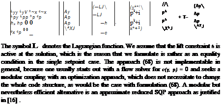
The matrix A denotes an appropriate approximation of the system matrix cx, which is used in the iterative forward solver. An algorithmic version of this modular for­mulation is given by the following steps


(1) generate hk by performing N iterations of an adjoint solver with right hand side fj (yk, pk) starting in hk

(2) generate ak by performing N iterations of an adjoint solver with right hand side hj (yk, pk) starting in ak

(3) compute approximate reduced gradients

g = fj + cjhk+1, y = hj + cp ak+1

(4) generate Bk+1 as an approximation of the (consistent) reduced Hessian

(5) solve the QP

B y]( &p = (-g Yj 0 pk+1 – h

(6) update pk+1 = pk + Ap

(7) compute the corresponding geometry and adjust the computational mesh

(8) generate yk+1 by performing N iterations of the forward state solver starting from an interpolation of yk at the new mesh.

This highly modular algorithmic approach is not an exact transcription of equation (69), but is shown in [16] to be asymptotically equivalent and to converge to the same solution. The overall algorithmic effort for this algorithm is typically in the range of factor 7 to 10 compared to a forward stationary simulation.

Now we generalize this algorithmic framework to the semi-infinite problem for­mulation (23-25). Numerical approaches to this problem class have already been proposed in [2, 3, 4].

For the sake of simplicity, we restricted the formulation to a problem with two set-points coupled via the objective, which is a weighted sum of all set-point object­ives (weights: ю1, (o2), and via the free optimization variables p, which are the same for all set-points. The generalization to more setpoints (i. e., the adaptive sparse grid points below) is then obvious. The lift constraint is formulated for the smallest value smin of all grid points. The corresponding Lagrangian in our example is

2 2

L (У1, У2, p, h,h) = Zfi, p, ^) + p, si )+ph(ymin, p, smin) (70)

i=1 i=1

The approximate reduced SQP method above applied to this case can be written in the following form

О

о

о

о

о

Ay1^

(-LA

0 0 0 0 0 Aj

Ay2

00 B y cjp cj, p

Ap

-Lj

О

о

о

Г*"

о

о

Ар

-h

о

о

о

о.

о

о

Ah

-c1

0 A2 c2,p 0 0 0

уАА2

-c2

We notice that the linear sub-problems involving matrices Aj are to be solved inde­pendently, and therefore trivially in parallel. The information from all these parallel adjoint problems is collected in the reduced gradient

2 2

g = + Ecj

i=1 i=1

Next, the solution of optimization step

"B n]( ap = f-g

Yj 0 pk+1) -hJ

is distributed to all approximate linearized forward problems

AiAyi + Ci, pAp = – Ci,

which can then again be performed in parallel.

Adaptive Sparse Grid

Since the function evaluations are very expensive in our application, we introduce in this section an adaptive sparse grid strategy in order to further reduce the number of grid points but conserving the approximation quality. The presented isotropic Smo – lyak algorithm is effective for problems whose input data uniformly depend on all dimensions. But the convergence rate deteriorates for highly anisotropic problems, such as those appearing when the input random variables come from a Karhunen – Loeve-Expansion as in our application [9]. The reduction of computational effort can be achieved by using spatially adaptive or dimension-adaptive refinement [33], [14]. In order to develop adaptive schemes during the cubature process, the inter­polation error can be used as an adaptivity indicator. Therefore, nested cubature formulas are useful since they allow the error evaluation based on the difference of two subsequent formulas. Due to the fact that in our application the mean value is computed by the sparse grid interpolation, this target value is also used as an error indicator for the adaptivity. The dimension-adaptive quadrature method tries to find important dimensions and adaptively refines in this with respect to given error es­timators. This leads to an approach which is based on generalized sparse grid index sets [14]. This strategy allows to employ every nested interpolation formulas, so it can be chosen problem dependent, e. g. in our application depending on the distribu­tion of the random variables. On the other hand, the locally refined sparse grid gives more flexibility in the adaptive procedure, but requires equidistant support nodes. In the following, we will discuss both strategies and compare the resulting sparse grids in the numerical results later on.

Подпись: Y1 Подпись: 0 for j = 1, m; = 1 2-^-1 for j= 1,...,пц,пц > 1 Подпись: (47)

Below, we introduce a locally adaptive hierarchical sparse grid approach using piecewise multilinear hierarchical basis functions following closely [27], [33]. Due to the straightforward implementation of the refinement, we choose the linear hat functions as interpolation basis functions which are also well established in the ad­aptive mesh refinement. The support nodes of the one-dimensional basis function are given by

with

Подпись:1, for і = 1

2 і-1 + 1 for і > 1

Подпись: a) (Y) Подпись: 1 -  {m, 0, Adaptive Sparse Grid Подпись: (49)

Hence, the interpolation formulas are defined by

The discussed univariate nodal basis functions (49) are now transformed into mul­tivariate hierarchical basis functions which are fundamental for the adaptive sparse grid. Considering once again the difference formula

f;(h) = Qi+1(h) – Q;(h) (50)

with

Q;(h)= X aj ■ h (Yj) (51)

Y) eGi

we obtain due to the fact that the support nodes are nested (e. g. G; c Gі+1) and accordingly Qі-1 (h) = Q; (Qі-1 (h)) the following representation of (50)

f;(h) = X a) ■ h (y;) – X aj ■ Q)-1 (h) (Y)) (52)

Y’eG Yj eG;

= X a1) ■ (h (y;) – Q)-1 (h) (Yj)) (53)

= X a) ■ (h(Yj) – Q)-1 (h) (Yj)) (54)

Y)G

since h(Y;) – Qi-1(h)(Yj) = 0, yYj e G)-1. Renumbering the elements in Gf = G; Gі-1, with mf = #Gf = m; – m1, leads to

mf

Al(h) = І a) ■ (h(Y)) – Ql-1(h)(Y[)). (55)

j=1

We define wl) = h(Yj) – Q1-1 (h) (y)^ as the 1D hierarchical surplus [6] which is the difference between the current and previous interpolation level. If the 1D Grid of level k interpolates the function h exactly, wk) is equal to zero for all j. So, this value can be used as an error indicator for each inserted grid point, since the hierarchical surpluses tend to zero as the level k tends to infinity (for continuous functions). Considering now again the multi-dimensional case, we obtain the sparse grid (46) in hierarchical form applying the derived formula of A i.

5(k, d)(f)= S(k – 1,d)(f)+ І (Al1 ®-‘®Ald) (f) (56)

|i|=k

= S (k – 1, d)(f ) + AS (k, d)(f) (57)

with

AS(kd)(f)= І І Wn®”’®)) ‘

|i|=*jtBi’—————— V———– ‘

aj

, , , , 44 (58)

(f(^:-’Y)d) -S (k -1d)(f) (и–®))

‘————————- v———————— ‘

wj

where Bi := {j є NN : YІ e G‘A for )l = 1,…, ml&,k = 1,…, d} is a new set of

multi-indices consistent with the multivariate hierarchical basis {aj: j e Bl, l < i}.

Thus, the objective function in our application can be approximated by the fol­lowing rather abstract expression:

f(P, Wd(Z))= І І wj(p) ■ aj(Z) (59)

|i|<k jeBi

The mean value of the objective function can be then computed as:

en (f (p))= І І wj (p) ■( aj (Wd(Z)) dP (Z) (60)

|i|<k jeBi Jn

where

! f1 ■ l, if l= 1

a) {Y))dY = < •/, if г = 2, (61)

21-1 ■ l, otherwise.

where l denotes the length of the given 1D interval, that means in our example l = 2. Instead of using the hierarchical surplus wij as an error indicator for the adaptivity (cf. [27], [33]), we suggest to adapt the grid checking the following expression:

wj := wj • aj (щ (Q) dP (Z) (62)

Since it is not necessary to exactly interpolate the drag depending on the uncertainty in the optimization loop in our application, the introduced adaptivity indicator wj only measures the difference between the value of the mean inserting a new point Yj of the current level of interpolation and the corresponding value of the mean at the previous interpolation level. The resulting algorithm in order to construct the sparse grid which is then used for the optimization slightly differs from [27], [33] due to the modification in the adaptivity indicator.

Adaptive Sparse Grid for High-Dimensional Integration

The mean value of the robust optimization problem depending on the current design vector is required in each iteration of the optimization algorithm. Since we can­not solve this integral analytically, we have to approximate it in appropriate, effi­cient way. Several possibilities can be found in the literature, the most common are: Monte-Carlo simulation, respectively general sampling methods, full tensor grid in­terpolation and sparse grid interpolation. Their efficiency depends on the dimension d of the probability space Qd and on the properties of the integrand f (y, p, yd). Each of these methods provides an approximation En of the mean value E( f) by evaluating the function f (y, p, yd) in N integration points yj, •••, Wn and summing the results f (yi, p, yld) multiplied with the weights 03, •••, (0N up

N

En = ^Юі • f (yi, p, yd) (38)

i=l

The sampling methods randomly select realizations of the uncertainties in the given probability space and take some kind of average of the function values at these points which converges to the exact value of the integral due to the law of large numbers. The advantage of this approach consists of the straightforward implement­ation, the algorithm only needs the underlying integration space as input and func­tion evaluations at the randomly selected points. But on the other hand, the expected convergence rate 0(N~2) requires a large number of function evaluations to ensure a given error tolerance. In our application, one function evaluation is very expensive since the solution of the flow equation, Euler or Navier Stokes equation, is needed. So, the sampling methods, even the improved methods which use additional inform­ation in order to select the realizations, are not an appropriate choice in our case to compute the mean value in our optimization problem.

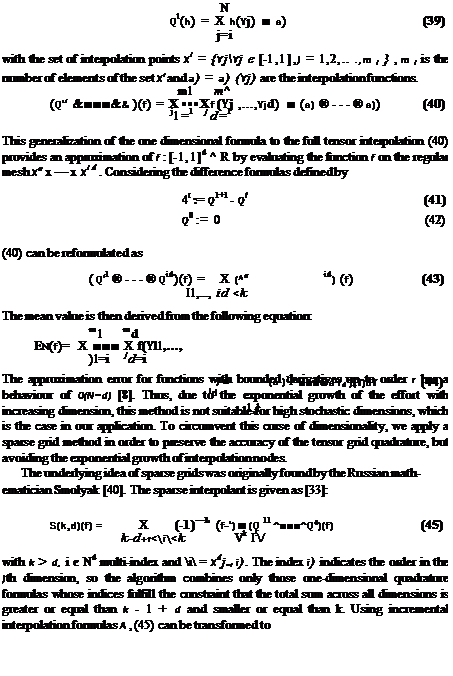
Another possibility obtaining the objective value is the full tensor grid quadrat­ure derived from the full tensor product of the one-dimensional interpolation for­mulas. Constructing the multi-dimensional interpolation, we first consider the fol­lowing one-dimensional interpolation formula in order to approximate a function h : [—l, l] ^ R:

Adaptive Sparse Grid for High-Dimensional Integration

5(k, d)(f) = X A1 (f)

i<k

= S(k – 1,d)(f) + X A1 ®—®Ad) (f)

i=k

with A = Ql+l – Ql, Q° = 0 and S(d – 1, d) = 0. The collection of all the interpol­ation points ( )

H (k, d) = У (X11 x—xX‘d) (46)

k—d+1<i<k

is called a sparse grid of level k.

The derivation of the sparse grid suggests the use of nested interpolation func­tions due to the recursive construction. In the literature, the most popular choice of the collocation points is the Clenshaw-Curtis grid at the non-equidistant ex­trema of the Chebyshev polynomials and the underlying interpolation formula is the Chebyshev-Gauss-Lobatto formula.

Reduction of the Dimension of the Probability Space Using a Goal-Oriented Karhunen-Loeve Basis

The evaluation of the objective function in the robust optimization problem (23) requires the computation of the mean, i. e. the computation of the integral of the random field with respect to its probability measure. Applying the introduced Karhunen-Loeve-Approximation, the objective function can be written as the fol­lowing d-dimensional integral

E (f (y, p, V(x Z)))= / ••• / (f (y, p, V(x Yi(Z),…,Yd (Z)))dYi(Z) • •• dYi(Z) n n

(36)

where d/і (Z) is the one-dimensional Gaussian measure. So, one term more in the truncated Karhunen-Loeve expansion to increase the approximation accuracy res­ults in an integral of one-dimension higher. In order to reduce the computational effort, the orthogonal basis functions {zi} will be chosen goal-oriented, i. e. the indi­vidual impact of the eigenvectors on the target functional will be taken into account. This method is well established in the model reduction methods of dynamic sys­tems and the adaptive mesh refinement (cf. [1]). The idea is to develop an error indicator for the individual eigenvectors reflecting the influence on the drag. The in­troduced error analysis of the Karhunen-Loeve-Expansion in section 2.2 only gives the approximation error of the random field ^, but not of the function of interest

Подпись: ПІ : Подпись: d/ dzi Подпись: dZi + dZi’ Подпись: УІ = Подпись: (37)

f (y, p, y). We propose to use sensitivity information to capture the local sensitivit­ies of the drag with respect to the eigenvectors

where X solves the adjoint equation. The adjoint equation is independent of i, hence it has to be solved only once and the indicator pi is numerically cheap to evaluate. Now, the reduced basis {z} can be automatically selected, the eigenvector zi with a large value n have to be kept in the reduced basis, whereas a small value indicates that the basis vector can be rejected from the basis.

Chance Constraint Formulations

Chance constraints leave some flexibility with respect to the inequality restrictions (cf. Ref. [37]) . The inequality restrictions are only required to hold with a certain probability P0

min f(y, p, s(Z))dP (Z) (29)

y, p

n

s. t. c(y, p,s(Z))= 0, VZ Є n (30)

P({Z Ih(y, p,s(Z)) > 0}) > P0 (31)

Chance Constraint Formulations Chance Constraint Formulations

So far, chance constraints are used mainly for weakly nonlinear optimization prob­lems Ref.[22, 20] . In the context of structural optimization (which is typically a bilinear problem), this formulation is also called reliability-based design optimiza­tion. For more complex problems, we need again some simplification. In Ref.[38] this is performed by applying a Taylor series expansion about a nominal set-point s0 := E(s), which is assumed to be equal to the expected value of the random vector s. Suppressing further arguments (y, p) for the moment, the Taylor approximation of 2nd order of f in (29) gives

Integrating this, we observe

E(/) = / f(s)dsP(Z) = f(s°) + £ ^p. Var{Si)

n i=1 i

where Var(si) is the variance of the ith component of s. Obviously, a first order Taylor series approximation would not give any influence of the stochastic inform­ation, which is the reason, why we use an approximation of second order for the objective. In order to deal with the probabilistic chance constraint (31), we also have to approximate its probability distribution. Since the uncertainties are all as­sumed to be Gaussian and truncated Gaussian, respectively, we use a first order Taylor approximation of the inequality constraint, since we know that this is again Gaussian and truncated Gaussian distributed (unlike the second order approxima­tion) (cp. Ref.[17] )

«И:=й(Л + ^(*-Л ~ («(/), ОЙ 1„,

where we assume for simplicity that h is scalar valued.

Chance Constraint Formulations
Now we can put the Taylor approximations together and achieve a deterministic optimization problem. Since the flow model (30) depends also on the uncertainties s, we should be aware that the derivatives with respect to s mean total derivatives. We express this by reducing the problem in writing y = y(p, s) via (30).

P({Z 1 h(y(p, s(Z)),s(Z)) > 0}) > po
^ P({Z 1 h(y(p, s(Z)),s(Z)) < 0}) < 1 – p0

The propagation of the input data uncertainties is estimated by the combination of a Second Order Second Moment (SOSM) method and first order Taylor series ap­proximation presented for example in Ref.[38]. Since there is no closed form solu­tion for the integral, the chance constraint is evaluated by a numerical quadrature formula.

Considering geometry uncertainties, a high amount of computational effort arises due to the high dimensionality of the resulting robust optimization problem. In the following, we will introduce two techniques in order to reduce the complex­ity of the problem: a goal oriented choice of the Karhunen-Loeve basis reducing the dimension of the probability space and (adaptive) sparse grid methods in order to efficiently evaluate the high dimensional integrals.