Our heavyweight helicopter equal in the world does not have
In Rostov started production of the most load-lifting rotary-wing car The Russian holding «Helicopt[...]

Everything about aircrafts and helicopters. News and events in aviation worldwide. Civil, transportation, military helicopters and airplanes.

Everything about aircrafts and helicopters. News and events in aviation worldwide. Civil, transportation, military helicopters and airplanes.

Everything about aircrafts and helicopters. News and events in aviation worldwide. Civil, transportation, military helicopters and airplanes.

Everything about aircrafts and helicopters. News and events in aviation worldwide. Civil, transportation, military helicopters and airplanes.


Oftentimes, the surface geometry one encounters does not fit a separable coordinate system. For these cases, the surface Green’s function usually cannot be found easily. For such a surface geometry, one may use the adjoint Green’s function and the reciprocity relation.
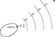
In many branches of mechanics, the reciprocity principle applies. However, the existence of a reciprocity principle has not been fully exploited in the fields of acoustics and fluid dynamics. Some earlier works that utilized reciprocity are Cho (1980), Howe (1975,1981), Dowling (1983), and Tam and Auriault (1998) in acoustics; Roberts (1960), Eckhaus (1965), and Chardrasekhar (1989) in hydrodynamic stability; and Hill (1995) in receptivity problems. To fix ideas on reciprocity, consider a time periodic point source of sound located at xs as shown in Figure 14.5(a). Let G(x0, xs, a) be the pressure associated with the sound field measured by an observer at x0. The time factor e-iat has been omitted. Mathematically, G(x0, xs, a) is the Green’s function of the Helmholtz equation and a is the angular frequency of oscillations. (Note: the notation that the first argument of the Green’s function is the location of the observer and the second argument is the location of the source is retained here.) Now, if the location of the sound source and that of the observer is interchanged as shown in Figure 14.5(b). Clearly, by symmetry, the pressure measured by the observer now at xs while the source is at x0 is the same as before. That is,
G(x0, xs, a) = G(xs, x0, a). (14.43)
Eq. (14.43) is simply a statement that the Green’s function G(x0, xs, a) is selfadjoint. It is the reciprocity relation.
Figure 14.5. An acoustic source and an observer form a self-adjoint system.

 |
X
Observer at x
s
For a surface source and a far-field observer as shown in Figure 14.6(a) a reciprocity relation exists. The problem is, however, not self-adjoint. The adjoint Green’s function is not governed by Eqs. (14.8) and (14.9). The boundary condition is not Eq. (14.10). These equations, referred to as the adjoint equations, may easily be derived in the frequency domain.
 |
![]()
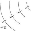
There is a significant advantage in using adjoint Green’s function instead of the direct Green’s function when an analytical formula for the Green’s function cannot be found. Suppose the far-field sound in the direction of в produced by surface sources as shown in Figure 14.7a is to be found. To determine the total far-field radiation, the radiation from each surface sources such as A, B, and C in Figure 14.7 has to be calculated and then summed. That is, the surface Green’s functions at A, B, and C and other surface points have to be separately computed. In the absence of an analytical formula, this would be a tedious and laborious effort. On the other hand, if
![]()
|
|
|
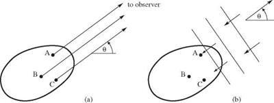
the adjoint formulation is used the situation is different. Since the source point is now in the far field, the sound waves from the far-field source near surface Г are plane waves. The adjoint Green’s function is, therefore, the solution of a simple scattering problem by surface Г. The scattering problem needs to be computed only once. By the reciprocity relation, the values of the direct Green’s function for radiation from every point on surface Г to the far-field point is found simultaneously in one single calculation of the scattered wave solution.
The Fourier transform of Eqs. (14.8), (14.9), and boundary condition (14.10) in time t are
— iop0V(g) + V p(g) = 0 (14.44)
– iop(g) + yP0V ■ v(g) = 0, (14.45)
On Г or 5 = 50,
p(g(x, op $0, П0, 50, t) = 2ns($ — $0Жп — П0Ушг (14.46)
To find the adjoint system of equations to Eq. (14.44) and (14.45), multiply Eq. (14.44) by v(a)■ and Eq. (14.45) by p(a) (the superscript “a” denotes the adjoint) and integrate over all space outside Г. This yields, after rearranging the terms,
![]() [—iop0v(a) ■ v(g) + V ■ (p(g)v(a)) — p(g)V ■ v(a) — iop(g)p(a))
[—iop0v(a) ■ v(g) + V ■ (p(g)v(a)) — p(g)V ■ v(a) — iop(g)p(a))
+ Yp0V ■ (p(a)v/(g) — yp0v(g) ■ Vp(a)]dxdydz = 0. (14.47)
The two divergence terms in Eq. (14.47) may be integrated by means of the Divergence Theorem to become surface integrals over Г. This leads to
flfi —iop0v(a) — yp0Vp(a)] ■ v(g)dxdydz
outside Г
+ i-i°p’«
outside Г
V ■ v(a)]p(g)dxdydz
— U [p(g)v(a) + Yp0p(a)v(g)] ■ n dS = 0.
surface Г
where n is the unit outward pointing normal of surface Г.
Now, the adjoint system is chosen to satisfy the following equations and boundary conditions:
|
– irp0v(a) – Yp0 Vp(a) = 0 |
(14.49) |
|
irp(a) – V ■ v(a) = 2nS(x – x1 )eirT |
(14.50) |
|
On Г or g = g0, p(a) = 0. |
(14.51) |
By means of this choice of the adjoint system, the integrals of Eq. (14.48) may be easily evaluated. This gives the reciprocity relation as follows:
p(g)(x1;f0, П0> т) = т) (M.52)
where vf’1 = v(a) ■ ii is the component of the adjoint velocity in the direction of outward pointing unit normal ii. Thus, once the adjoint problem is solved, the direct surface Green’s function on the entire surface is found.
Instead of using surface pressure as the variable for continuation to the far field, an equally good variable to use is the velocity component normal to the surface or the normal pressure gradient. If this choice is made, the appropriate surface Green’s function is given by solution of the following problem (a superscript “G” will be used to denote this Green’s function):
|
д V(G) Po dt +VP(G) =o |
(14.25) |
|
djP^- + YPoV • v(G) = o, |
(14.26) |
On surface Г, i. e., g = go, the boundary condition is
![]() v(G)(x, t; to, no, So, to) = s(t — toЖп — По)Ж — to)•
v(G)(x, t; to, no, So, to) = s(t — toЖп — По)Ж — to)•
To find v^ (x, t; to, no, go, t), it is advantageous to introduce a velocity potential Ф(^ defined by
v(G) = v ф(^, p(G) = — po——- . (14.28)
dt
Eq. (14.28) satisfies Eq. (14.25) identically. Substitution of Eq. (14.28) into Eq. (14.26), the governing equation for Ф(^ is found to be
1 d 2ф^)
2 v2 Ф(^ = o. (14.29)
ao dt2
The surface boundary condition on g = go is found by inserting expression (14.28) into Eq. (14.27). This yields
дФ^)
-— = S(i — to )S(n — no )S(t — to), (14.3o)
where n is the unit outward pointing normal of surface Г.
Suppose Ф(С)(х, t; ^0,v0,g0, t0) is found. Let vn (f0, n0, t0) be the prescribed
normal velocity on Г, then the velocity potential (v = V Ф and p = — —дф) is
p0 dt
given by
TO TO TO
![]() /// Ф )(x, t; %0’ n0’ ?0’ t0)vn (^0’ n0’ t0) d^0 dn0 dt0- (14.31)
/// Ф )(x, t; %0’ n0’ ?0’ t0)vn (^0’ n0’ t0) d^0 dn0 dt0- (14.31)
-TO – TO – TO
The pressure field may be computed by differentiating Eq. (14.31) with respect to t, i. e.,
By means of Eq. (14.28), this expression may be rewritten as
To illustrate the construction and use of surface Green’s function p(G), consider again the case of Г in the form of an infinite circular cylindrical surface as shown in Figure (14.2). The governing equation for Ф(^ is Eq. (14.29). In cylindrical coordinates, the equation and boundary condition for Ф(^ are
At r = ^
ЭФ(С) = 3(ф – ф0)8(x — xQ)8(t -10) 9 r D/2
Just as in Section 14.2, the solution of this problem may be constructed by first applying Fourier transforms to x and t and then expanding the solution as a Fourier series in (ф — ф0). On denoting the Fourier transform by a ~ over the variable and the amplitude function of the mth term in the Fourier series by a subscript m, the solution takes on the following form:
TO
Ф(G) = Фтеіт(ф—ф0). (14.36)
— TO
It is straightforward to find that
where H<m) and Hm are the mth order Hankel function and its derivative. The
inverting the Fourier transforms, it is readily found that
 |
||
Ф(G)(r,<p, x; фо, Xq, to)
For radiation to the far field, the k integral in Eq. (14.37) may be evaluated asymptotically (method of stationary phase) by first switching to spherical polar coordinates as in Section 14.2. In so doing, and upon using Eq. (14.28), it is found that
p (а)(Я, в,Ф, t; Фо, Xq, to)
R^to
To demonstrate that Eq. (14.38) is the correct surface Green’s function with vn as the matching variable, the time periodic monopole source problem of Section 14.2 is again considered. For a monopole source located at the origin with angular frequency Q, the pressure field is given by Eq. (14.19). By means of the radial (R direction) momentum equation, it is easy to find that the radial velocity vR associated with the acoustic field is
The component of vR in the direction normal to the cylindrical surface and on the cylindrical surface, r = D/2 is
where R0 = (D + x2 )1/2 and sin в = D. x0 and t0 are the source coordinate and time.
Now, on inserting p(G) from Eq. (14.38) and vn from Eq. (14.40) into Eq. (14.33), the radiated pressure field at R ^ to is given by
p (R, в, ф, t)) =
 |
R^to
The integrals over dt0 and dф0 can easily be evaluated to yield
ю 2n
I e*(“-Q)to dt0 = 2nS (a – Q), J eim(^—фо^ф0 = 2П ^.
-ю 0
 |
|
Thus, upon integration over dt0, d(p0, and da and on summing over m, Eq. (14.41) becomes
The remaining integral of Eq. (14.42) can be evaluated in closed form by differentiating formula (14.23) with respect to parameter a. By means of this formula, it is easy to find that the pressure field becomes
iQ R-t
This is just the acoustic field of a time periodic monopole.
Eqs. (14.1) and (14.2) are linear. The solution of these equations satisfying boundary condition p = pEuler on surface Г can be found by means of a Green’s function. For clarity, a superscript “g” is used to denote the variables of the Green’s function. Let (f, n, s) be a set of body-fitted curvilinear coordinates. The surface Г corresponds to g = g0. The Green’s function (v(g), p{g)) satisfies the following boundary value problem:
d v(g)
Po—~ + V p(g) = 0 (14.8)
dt
+ YPqV ■ v(g) = 0 (14.9)
dt
On Г, i. e., g = Sq,
p(g)(x, t; fo, no, So, to) = S(f – fo)S(n – По)S(t – to) (14.10)
(Note: The notation that the first set of spatial and time argument of the Green’s function represents the location and time of the observer while the second set represents that of the source is adopted here.)
When the Green’s function is found, the far-field pressure is given by
TO
p(x, t) = /// p(g) (X, t; fo, no, g0, t0)pEuler(f0, n0, g0, t0)df0 dn0 dt0• (14.11)
— TO
As an example of the use of surface Green’s function, the case of Г in the form of an infinite circular cylindrical surface of diameter D (see Figure 14.2) is considered. The cylindrical coordinates (r, ф, x) are the natural body-fitted coordinates of this problem. By eliminating v(g) from Eqs. (14.8) and (14.9) in favor of p(g) and upon applying Fourier transform to t, the time variable, the governing equation for p (the Fourier transform of p(g)), is found to be
|
|
 |
 |
||
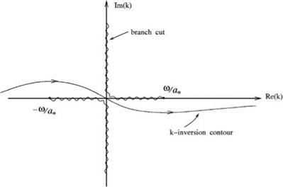
The solution of Eq. (14.15) satisfying boundary condition (14.16) can easily be found in terms of Hankel function []. On inverting the Fourier transform in x and the sum over n, it is found that
The branch cuts for the square root function (k2 – 4-) 2 in the k plane is shown
a0
in Figure (14.3).
For radiation to the far field, it is advantageous to switch to polar coordinates (Я, в,ф) (see Figure 14.4) with
x = R cos в, r = R sin в
 Figure 14.4. Spherical polar coordinates (R, в, ф), cylindrical coordinates (г, ф, x), and Cartesian coordinates (x, y, z).
 |
||
For large R, the Hankel function in the numerator of Eq. (14.17) may be replaced by its large argument formula. The к – integral can then be evaluated by the method of stationary phase. Upon inverting the Fourier transform in t, the far field Green’s function is found to be
(14.18)
As a simple demonstration that Eq. (14.18) is the correct surface Green’s function, the case of a sound field produced by a time periodic monopole of angular frequency L located at the origin of coordinates is considered. The pressure field is
where R is the radial distance. On the cylindrical surface of diameter D, the polar distance is R = (D – + x2)1/2 for a point at x = x0. Thus, the fluctuating surface pressure is given by
![]() (14.2o)
(14.2o)
By inserting p(g) from Eq. (14.18) and p(x0, ф0, t0) from Eq. (14.20) into Eq. (14.11), the far-field pressure due to surface pressure on the cylindrical surface is
|
+ x2) Ho(1)(fDsm в) |
The right side of Eq. (14.21) may be integrated step by step as follows. Integration over dф0 is zero except for n = 0. In this case, the integral is 2n. Integration over dt0 gives 2nS(m — L). Therefore, on integrating over dm, the right side simplifies to
Now, from the extensive compilation of Fourier integrals of Erdelyi et al (1954), the following closed-form integral is found:
![]() n eib(x2+a2)1/2—iyx
n eib(x2+a2)1/2—iyx
f (x2 + a2)1/2 dX = ІПH0(1) [a(b2 – У2)1/2] •
—r
By means of Eq. (14.23), it is straightforward to simplify Eq. (14.22) to
Thus, the monopole sound field at large R is recovered.
Consider the acoustic field generated by some localized noise sources as shown in Figure 14.1. The sound field is governed by the compressible Navier-Stokes equation. Suppose the solution is known. To identify that it is the solution of the Navier-Stokes equations, a subscript NS will be added to the pressure and velocity field, i. e., pNS and vns.
Now let y be a convex surface enclosing the sources and the near sound field. It will be assumed that y is far enough away from the sources that the disturbances at Y are, for all intents and purposes, linear and inviscid. Under these conditions, the equations of motion outside y are the linearized Euler equations as follows:
Thus, in the region outside y, PNS, vNS and the solution of the linearized Euler equations, denoted by pEuler, vEuler are practically the same, namely pNS ^ PEuler,
vNS ^ vEuler.
Suppose Г is a closed convex surface enclosing y as shown in Figure 14.1. On Г, P = PEuler is known. Now, as a first step toward establishing a way to continue the
solution from surface Г to the far field, consider the following initial boundary value problem in the space outside Г. The governing equations are the linearized Euler equations (14.1) and (14.2). The boundary and initial conditions are as follows:
on Г, p = PEuler (14.3)
At |x| ^ to, p, v behave like outgoing waves (14.4)
At t = 0, p = PEuler (X, °), V = VEuler (X, °) (14.5)
By eliminating v from Eqs. (14.1) and (14.2), the equation for p is the simple wave equation as follows:
d2 p
-2- – «0V2p = (14.6)
Now, it is known that the solution of the simple wave equation (14.6)) satisfying boundary conditions (14.3) and (14.4) and initial conditions (14.5) is unique, but the original solution pNS, vNS which become pEuler, vEuler outside Г is also a solution of Eq. 14.6 and boundary and initial conditions (14.3) to (14.5). Therefore, the two solutions must be equal. In other words, the continuation solution from surface Г to the far field is given by the solution of Eqs. (14.1) to (14.5). Hence, a way to continue a near-field solution to the far field is to solve the initial boundary value problem stated above. How to construct such a solution is the subject of the next few sections of this chapter.
Instead of specifying p = pEuler on Г as boundary condition, the solution of the simple wave equation with dp = apEukI (the normal derivative) specified as boundary condition on Г is also unique. By Eq. (14.1), the normal derivative of p is related to the velocity component in the normal direction as follows:
^ d V „ d Vn
Vp • n=-P0 — ■ n=-P0-df • (14J)
However, if vn (x, t) is known on Г, then is known. Therefore, it is possible to
extend or continue a solution beyond surface Г by solving Eqs. (14.1) and (14.2) with appropriate initial conditions and matching vn to vnEuler on boundary Г. In other words, there are two ways to continue a solution from surface Г to the far field. The first way is to match p on Г. The second way is to match vn on Г.
It is worthwhile to note that the solution to the initial boundary value problem defined by Eqs. (14.1) to (14.5) consists of two parts. One part is associated with the initial conditions and zero boundary values on Г. The other part is the zero initial conditions and nonzero boundary value on Г. In most problems, interest is on the second part of the solution at large time. At large time, the transient solution (the first part) would propagate away. So for a long time solution, it is possible to ignore the initial condition altogether. In the rest of this chapter, attention is focused only on continuing the solution from surface Г without reference to initial conditions.
In the literature, there are currently two favorite methods for continuing a solution to the far field. They are the Kirchhoff method (see, e. g., Lyrintzis (2003)) and the Ffowcs-Williams and Hawkings (1969) integral method. Mathematically, the Kirchhoff method yields a far-field acoustic pressure in terms of an integral
over a closed surface. The integral involves the values of the pressure, its normal derivative, and the time derivative on the closed surface (three quantities altogether). This is well known to physicists and mathematicians. The Ffowcs-Williams and Hawkings method is similarly a surface integral representation. It solves the Lighthill equation instead of the simple wave equation. If the surface under consideration is outside all volume sources (quadrupoles), then the Kirchhoff method and the Ffowcs-Williams and Hawkings method are essentially similar. It is to be emphasized that both are integral representations, not solutions of the governing equations. To evaluate the integrals, the values of the pressure, its normal derivative, and time derivative on the surface must be known. It will, however, be shown later that it is sufficient to continue the pressure field from surface Г to the far field by using only the pressure fluctuations on the surface. Alternatively, it is sufficient to determine the far-field pressure by using the fluctuating pressure gradient or the velocity component normal to the surface. It is not necessary to have three or more sets of information. This, nevertheless, does not mean that the Kirchhoff and the Ffowcs-Williams and Hawkings methods are in error, only that when these methods are used, the prescribed pressure, its normal derivative, and time derivative on surface Г must be accurate. Otherwise, because of the overspecification of the boundary data (Note: in the theory of partial differential equations, when two sets of boundary data are prescribed, whereas one set is sufficient for determining a unique solution, it is referred to as overspecification of boundary data), the computed far – field pressure is likely to incur significant error.
By now, it is abundantly clear that all computational aeroacoustics (CAA) simulations can only be carried out in a finite, and in most cases, as small as possible, computational domain. A critical problem is how to continue the numerical solution to the far field. In some cases, the acoustic field consists of discrete frequency sound or tones. But in most cases, such as jet noise, the sound field is broadband and random. In aeroacoustics, most broadband noise is the result of turbulence. Turbulence is random and definitely nondeterministic, and the same is true of the radiated noise. The nondeterministic nature of the noise of turbulence makes its continuation to the far field a much more challenging task.
Mathematically, the problem of extending a near-field acoustic solution to the far field is akin to the mathematical procedure of “analytic continuation” in complex variables. Analytic continuation extends an analytic function defined in a limited domain to a large domain. Because the ideas behind the two problems are similar, the word “continuation” is used here to indicate the objective and intent.
At high Reynolds numbers, a flow is inevitably turbulent. As noted earlier, a turbulent flow is chaotic and random. For a turbulent flow such as that of a high Reynolds number jet, the solution is nonunique. Nonuniqueness is a characteristic of turbulence. Only the statistical averaged quantities are stationary with respect to time. This being the case, it brings forth the question of what physical variables should be continued to the far field. There is also the question of cost in performing the continuation. One may wish to continue the entire turbulence information to the far field, but the computational cost is likely to be prohibitive. Thus, this may not be a good idea. From a practical standpoint, the crucial information one needs in the far field is the noise directivity and spectra. If, indeed, the noise spectra and directivity are the information required in the far field, then a not so expensive computational procedure may be developed to continue this information from the near to the far field. In this chapter only the continuation of the spectra and directivity of turbulence noise are considered.
Turbulent flows are nonlinear, but outside the turbulence region, the velocity and pressure fluctuations are essentially linear. According to the investigation of Phillips (1955) and Stewart (1956), the mean squared fluctuating velocity associated with a turbulent jet or a similar flow decays with an inverse fourth power of the distance from the turbulence region. This prediction has been confirmed by Kibens (1968),
Figure 14.1. Sound generated by a localized source.
 Bradbury (1965), and Maestrello (1973) experimentally. Outside the turbulence region, where the linearized Euler equations are valid, the mean squared velocity fluctuations decay with a second power with distance. This is the beginning of the acoustic near field. It will be assumed that the turbulent flow computation extends beyond the turbulence-irrotational boundary to the acoustic near field in the physical domain. The task of interest and the principal objective of this chapter are to develop a robust computational method to continue the numerical solution from the acoustic near field to the far field.
As an example of the use of overset grids in three dimensions, consider the propagation of a small-amplitude three-dimensional spherically symmetric acoustic pulse across a sliding interface. This problem is chosen because an exact solution
(linearized) is available for comparison. On taking into account spherical symmetry, the linearized dimensionless momentum and energy equations are
![]()
 |
9 p 1 d 2
+ (R2v) = 0,
dt R2 dR
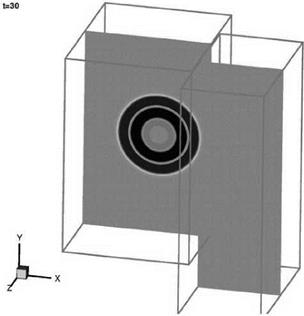
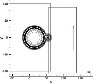
Figure 13.23. Computed pressure contours in the x — y plane at t = 30.
 where R is the radial coordinate and v is the radial velocity. The initial conditions at t = 0 corresponding to a radially symmetric Gaussian pressure pulse with a half-width b are
![]()
![]()
 (13.47)
 |
(13.48)
The exact solution of Eqs. (13.49), (13.50), and (13.51), which is bounded at R = 0, is
Numerical computation of this problem in three-dimensional Cartesian coordinates using the 7-point stencil DRP scheme and the optimized multidimensional interpolation method for data transfer across the sliding interface has been carried out. This may be regarded as a three-dimensional extension of the acoustic pulse problem of Section 13.4.1. The major difference is that there are now 64 points, 4 x 4 x 4, in the interpolation stencil. Again, as in the two-dimensional problem, a
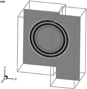
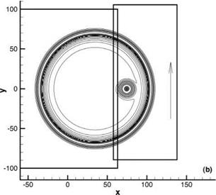
Figure 13.24. Computed pressure contours in the x — y plane at t = 60.
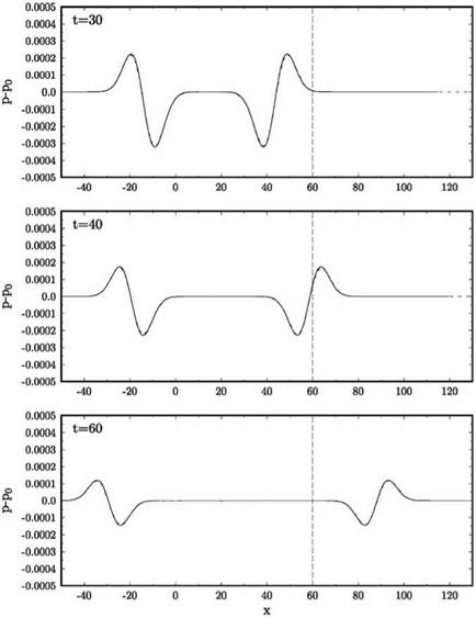
 uniform mean flow at Mach 0.5 in the x direction is included (the exact solution is obtained by applying a moving coordinate transformation to solution (13.52)). The sliding grid is taken to be moving in the z direction at a Mach number of 0.4. The full Euler equations are computed. The initial conditions are as given in Eqs. (13.47) and (13.48). The initial pressure pulse has a half-width of six mesh spacings and an intensity with e = 0.005. The pulse is centered at the origin of the coordinate system. The sliding interface is located at x = 60.
Figures 13.23 and 13.24 show the computed pressure contours in the x — y plane at time t = 30 and 60. The acoustic pulse expands spherically at a dimensionless speed
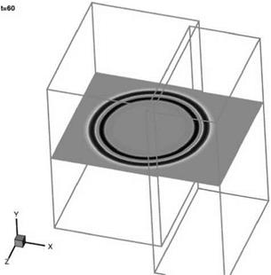 Figure 13.25. Computed pressure contours in the x — z plane at t = 60.
|
Figure 13.26. Comparisons of computed waveforms with exact solution at t = 30, 40, and 60. |
of unity and is simultaneously convected in the downstream direction by the mean flow at a speed of 0.5. At time t = 30, the pulse has not reached the sliding interface. At t = 60, part of the pulse has crossed the sliding interface into the downstream moving grid. The computed pressure contours remain circular. Figure 13.25 shows the pressure contours at t = 60 in the x – z plane. Again, the contours are circles centered at x = 30, z = 0. Figure 13.26 shows the computed wave form in the x – y plane at t = 30, 40, and 60. Plotted in this figure also are the exact wave forms, but they cannot be detected because they differ from the computed solution by less than the thickness of the lines.
Finally, it is worthwhile to point out that overset grids method may also be used for computing the solutions of moving boundary problems. In such applications, a stationary grid and a moving grid attached to a moving object are used. For this type of problem, the overlapping grids change constantly with time. As a result, a good deal of effort is needed in locating the overlapping grids.
EXERCISES
13.1. To find the values of P in Exercise 11.2, one may use the multidimensional optimized interpolation method. Compare the result of this method and the two – step line interpolation method of Exercise 11.2.
13.2. Use the overset grids method to compute the scattered sound field generated by a plane incident wave train impinging on two cylinders. An exact solution can be found following the method of Sherer (Proceedings of the Fourth CAA Workshop on Benchmark Problems, NASA CP 2004-212954, September 2004).
13.3. (A moving boundary problem) Sound is generated by an oscillating cylinder of diameter D immersed in an inviscid, non-heat-conducting gas. The center of the cylinder lies on the x-axis and is moving so that at time t it is located at x = F(t), where F(t) is a periodic function. One way to compute the radiated sound is to use the overset grids method. This will involve several steps.
Step (1). Use a cylindrical grid fixed to the cylinder as in Figure 13.2. In the cylinder-fixed coordinate system, the governing equations have to be derived by performing a change in coordinates to the Euler and energy equations. Let (xc, yc) be the cylinder-fixed Cartesian coordinates centered at the center of the cylinder. Then,
x = xc + F (t )> y = Ус-
The relationships between (xc, yc) and cylindrical coordinates (rc, Qc) are
xc = rc cos(0cX yc = rc sin(0c)-
Now, transform the Euler and energy equations to the cylinder-fixed coordinates. The value of (u, v, p, p) on the cylindrical mesh are computed by solving this set of equations. Note that u is still the velocity component in the x direction with respect to the background-fixed coordinates. If uc is the component relative to the cylinder, then, uc = u – dF.
Step (2). Use a Cartesian coordinates system to compute the values of (u, v, p, p) in the background coordinates. The background mesh has a square hole similar to that of Figure 13.1. This hole moves with the cylinder in the course of time.
Step (3). The values of (u, v, p, p) on the outer most three rings of the cylindrical mesh are not computed. They are obtained by interpolation from the values of those on the background mesh. Similarly, those values at the innermost three rows and three columns of the square hole are not computed. They are to be found by interpolation from the values on the cylindrical mesh.
Develop a computational strategy for performing the acoustic radiation computation.
Appendix 13A. Computation of the Values of the Elements of Matrix A as Xj ^ xk
As alluded to previously, when the stencil points are aligned on a coordinate line, the limit form of the matrix elements as given by Eqs. (13.16) and (13.20) are to be used; e. g.,
Д sin( )
lim ———————— = к.
Xi^Xk (xj – Xk)
However, for points very nearly aligned, direct numerical evaluation of the matrix or vector elements is not recommended because of the division by a small number. Instead, we advise that the limit values be used whenever |x;- – xk| < e. To find a suitable value of e, let us consider the error incurred when (Д/(х;- – xk))sin(K (x;- xk)/ Д) is approximated by its limit value к, where |x;- – xk| < e. Let Z = (x;- –
хк)/Д, we have by Taylor series expansion,
It is easy to establish
Thus, the relative error of using the limit value to approximate the relevant parts of a matrix element is less than (к2/3!)(е/Д)2. We recommend to take e/Д = 10-5 for к = 1.2. In this case, the relative error is less than 2.4 x 10⁻¹¹. This is an extremely small error.
Appendix 13B. Derivation of an Exact Solution for the Scattering of an Acoustic Pulse by a Circular Cylinder
In this appendix, an exact analytical solution for the scattering of an acoustic pulse by a circular cylinder is derived. The solution provided in the Proceedings of the Second CAA Workshop on Benchmark Problems has an error.
Let the cylinder be centered at (x, y) = (0, 0) with a radius r0 and the acoustic pulse be initialized as
p(x, y, 0) = e-b[(x-Xs)2+(y-ys)2], u = v = 0 at t = 0, (13.53)
where p is the pressure, (u, v) is the velocity, and b = (ln2)/d2. Here, d is the halfwidth of the pulse, and (xs, ys) is the center of the initial pulse. The solution will be found in terms of a velocity potential ф defined as
Let
Ф(Х, y, t) = Фі(x, y, t) + Фг(x, y, t),
where Фі(х, y, t) represents the wave generated by the pulse in the free space and Фг(х, y, t) represents the wave reflected by the cylinder. The solution for Ф(х, y, t) is
TO
![]()
![]() j Ai (x, y, ш) e~iotdo 0
j Ai (x, y, ш) e~iotdo 0
where
and rs = у (x – xs)2 + (y – ys)2. Here, Im{} and Re{} denote the imaginary and real part of {}, respectively, and Jk denotes the Bessel function of order k.
To find Фг, on following Eq. (13.55), the solution may be taken to have the following form:
in which Ar(x, y, ш) satisfies the Helmholtz equation
and the following solid wall boundary condition on the cylinder,
Ar can be solved by separation of variables in the polar coordinates (r, в), which gives the following expansion: (ys = 0)
TO
Ar (x, y, oj) = ^2 Ck (ш) Hk ) (roj) cos (кв). (13.59)
k=0
 |
In Eq. (13.59), H(1) is the Hankel function of the first kind of order k. The expansion in Eq. (13.59) ensures that Фг will satisfy the far-field radiation condition. Then, the boundary condition Eq. (13.58) leads to
(13.60)
where
where e0 = 1 and ck = 2 for k = 0.
Finally, the total pressure field can be found as follows:
TO
![]() J (At(x, y, ю) + Ar(x, y, m))me-imtdm 0
J (At(x, y, ю) + Ar(x, y, m))me-imtdm 0
where Ai(x, y, ю) is given by Eq. (13.56) and Ar(x, y, ю) is given by Eq. (13.59).
![]()
13.4.1 Sliding Interface Problem in Two Dimensions
Aircraft engine noise is a significant environmental and certification issue. Noise generated by the fan rotor wake impinging on the stator is an important noise component at both takeoff and landing. In the Second CAA Workshop on Benchmark
Figure 13.17. Zero pressure contours at the beginning of a cycle. Pressure pattern formed by the scattering of a plane wave by a cylinder. Wavelength equal to quarter diameter of cylinder.
 Problems, a simplified model of this noise mechanism was proposed as a benchmark problem. One important feature of the problem is a sliding interface imitating the relative motion between a fan blade fixed computation domain and a stator blade fixed computation domain. Here, a less demanding sliding interface problem is considered. It will be shown that the use of an optimized interpolation scheme and overset grids method yields accurate numerical results.
 |
Figure 13.19 shows two computation planes with six columns of overlapping meshes. The left computation plane is stationary. The right computation plane moves upward at a velocity of vg. The sliding interface is the line at the center of the overlapping meshes. (x1, y1) will be used to denote the coordinates of a point in the stationary computation plane on the left, and (x2, y2) will be used to denote the coordinates of a point in the moving computation plane on the right. The relationships between the two coordinate systems are x2 = x1, y2 = y1 – vgt.
For computation purposes, square meshes are used in each computation plane, i. e., Ax1 = Ayx, Ax2 = Ay2 = 0.78Ax1. However, the mesh sizes are not the same in the two computation grids. Dimensionless variables with Ax1 as length scale, a0 (the speed of sound) as the velocity scale, Ax1/a0 as the time scale, p0 (mean flow density) as the density scale, and p0a2 as the pressure scale are used. It will be assumed that there is a uniform mean flow at 0.5 Mach number in the x direction over the entire computation domain. The x direction is the horizontal direction in Figure 13.19. The sliding interface is at x = 60.
The governing equations are the Euler equations. In the stationary computation plane, they are given by Eq. (13.1) with x replaced by x1 and y replaced by y1. In the moving computation plane, the governing equations, with respect to a grid fixed frame of reference, are:
d v d v 9 v 1 9 p
— + u— + (v — vg)— +—————- = 0
dt 9×2 g dy2 p dy2
 |
|
At time equal to zero, a pressure pulse centered at x1 = y1 = 0 is released. At the same time, a vorticity pulse and an entropy pulse centered at x1 = 40, y1 = 0 are released. Mathematically, the initial conditions at t = 0 are as follows:
where c = 0.005 and y = 1.4. In the course of time, the acoustic, the vorticity, and the entropy pulse will all be propagating or convected downstream. They will all reach the sliding interface at nearly the same time. They will then move across the sliding interface into the moving grid farther downstream. The exact solution of this problem was given in Section 6.4.
In the computation, the 7-point stencil DRP scheme is again used. For points on the stationary grid, the unknowns on every grid point including those on the sliding interface are determined at every time step by solving Eq. (13.1). Similarly, for points on the moving grid, the unknowns on every grid point including those on the sliding interface are updated according to Eq. (13.43). The unknowns of the three extra columns of grid points extending beyond the sliding interface are not calculated by the 7-point stencil DRP scheme. They are found by optimized interpolation using a 16-point stencil from the values of the variables on the other grid. In this way, information of the solution is passed between the two computation grids.
Figures 13.19a-13.19c show the computed density contours associated with the acoustic and entropy pulses at time t = 5.6, 44.9, and 73.0. In this computation vg is set equal to 0.4. Also plotted in these figures are contours of the exact solution in dashed lines. Because the difference between the computed and the exact solution is small, the dashed lines may not be easily detected. In Figures 13.19a, the two pulses are in the stationary grid. Figures 13.19b shows that the acoustic pulse, moving downstream at three times the velocity of the entropy pulse, catches up with the entropy pulse right at the sliding interface. Figures 13.19c shows that the entropy pulse has now been convected past the sliding interface onto the moving grid. At this time, the acoustic pulse has already propagated further downstream. Figure 13.20 shows the computed and the exact density waveform along the x-axis at four different times. The sliding interface is located at x = 60. It is clear from these figures that
|
Figure 13.20. Spatial distribution of density perturbation p’ = p — 1 associated with an acoustic and an entropy pulse propagating across a sliding interface located at x = 60. Dashed line is the exact solution. |
the treatment of a sliding interface using optimized interpolation is effective and accurate.
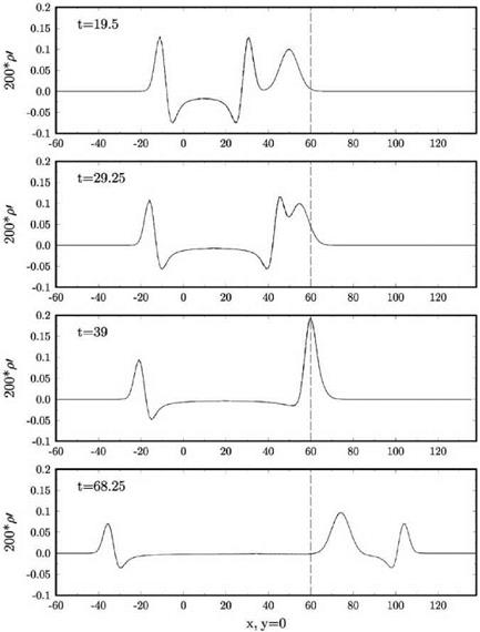
Figures 13.21a and 13.21b show the computed and the exact fluid velocity excluding the mean flow, (w/2 + v/2)1/2, contours of the acoustic and vorticity pulses as they propagate through the sliding interface. Again, the difference between the computed and exact contours, being less than the thickness of the contour lines, is difficult to detect. Figure 13.22 shows the waveform along the x-axis at four instances of time. At t = 29.25 to t = 39, the two pulses merge and propagate across the sliding interface together. At time t = 68.25, the acoustic pulse has passed through the entropy
Figure 13.21. Contours of fluid velocity (и’2 + v’2)1/2 associated with the transmission of an acoustic and a vorticity pulse across a sliding interface. Dashed lines are the exact solution. (a) t = 28.1. (b) t = 67.3.
 pulse and the two pulses are now separated. The computed waveforms are in good agreement with the exact solution.
In this computation, the moving grid moves at a subsonic velocity. In a similar computation the same results are recovered when the moving grid slides past the stationary grid at a supersonic velocity.
In a paper by Kurbatskii and Tam (1997), the problem of plane wave scattering by a cylinder was solved using a Cartesian boundary treatment method. Here, the same problem is solved using the overset grids method. One advantage of the overset grids method in this case is that the simple ghost point method may be used to enforce the
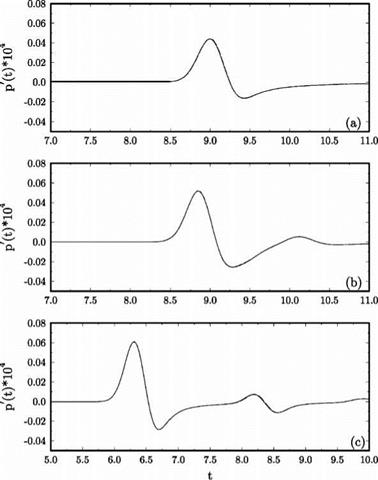
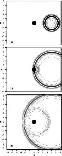
Figure 13.15. Pressure contours showing the scattering of an acoustic wave pulse by a circular cylinder. (a) t = 1.6. (b) t = 4.0. (c) t = 6.4. Dashed lines are the exact solution.
 wall boundary condition. Again, the 7-point stencil DRP scheme is used to solve the Euler equations. In order to be able to validate the numerical solution, the amplitude of the incoming waves with wave front perpendicular to the x-axis and wavelength equal to 8 Ax is set to be very small. The problem, therefore, is essentially linear and the accuracy of the computed solution can be ascertained by comparison with the exact linear solution.
Figure 13.17 shows the computed zero pressure contours at the beginning of a cycle. Plotted in this figure also are the contours of the exact solution in dashed line. The difference between the computed and the exact solution is very small; less than
|
Figure 13.16. Time history of pressure perturbation p’ = p — (1 /у ) at (a) x = -5, y = 0, (b) x = —4, y = —4, (c) x = 0, y = —5. Dashed line is the exact solution. |
the thickness of the lines. Figure 13.18 shows the computed and the exact scattering cross section а (в) defined by
__ 1
а (в) = lim rp2 2 , (13.42)
where the overbar denotes time average and ps is the pressure of the scattered acoustic waves. There is good agreement between the two. A major part of the small discrepancies arises because the computed result is measured at a finite distance from the center of the cylinder, whereas the exact solution is determined by taking the asymptotic limit r ^ to.
As examples to illustrate the use of overset grid method, two problems involving acoustic scattering by a rigid cylinder in two dimensions discussed in Section 13.1 will now be considered. The governing equations in Cartesian and cylindrical coordinates are Eqs. (13.1) and (13.2). They are discretized, and the numerical solutions are advanced in time by the 7-point stencil DRP scheme. The ghost point method is used to enforce the no-through-flow boundary condition.
13.3.1 Transient Scattering Problem
First, consider the scattering of an initial pressure pulse by the cylinder. For this problem, the Euler equations are solved with the initial conditions as follows:
 |
t = 0,
u = v = 0, p = ^1 — ^ + p
With a very small initial pulse amplitude (e = 10—4), the computed solution is identical to the solution of the linearized Euler equations. This cylinder scattering problem governed by the linearized Euler equation is a benchmark problem of the Second Computational Aeroacoustics (CAA) Workshop on Benchmark Problems. The exact solution given in the conference proceedings unfortunately has an error. The correct solution is provided in Appendix 13B at the end of this chapter.
|
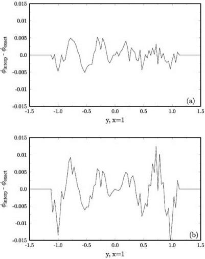
Figure 13.14. Distribution of interpolation error along the line x = 1. (a) Using a 16-point regular stencil in the r — в plane. (b) Using a 16-point irregular stencil in the x — y plane. |
Figure 13.15 shows the computed pressure contours at t = 1.6, 4.0, and 6.4. The computed contours and the contours of the exact solution are indistinguishable (the difference is less than the thickness of the contour lines). The direct acoustic pulse and the scattered pulse can clearly be seen in Figure 13.15. For a more comprehensive comparison between the numerical and exact solution, the pressure time history at three locations with Cartesian coordinates (—5, 0), (—4, 4), and (0, 5) are plotted in Figure 13.16. Plotted also in these figures is the exact solution. The differences between the exact (dashed line) and computed solution are again very small.
An interpolation stencil may be in the form of a regular stencil in a curvilinear coordinate system, but it would be an irregular stencil when a different coordinate system is used as the frame of reference. For example, Figure 13.4 shows a regular 16-point interpolation stencil of the polar coordinate system. That is, if the r – в plane is used for computation, the interpolation stencil points form a regular stencil. But, if the computation is done in Cartesian coordinates, namely the coordinates of the stencil points are specified in a Cartesian coordinate system, the interpolation points form an irregular stencil.
In overset grids computation and in other applications, extensive interpolation from one set of mesh points of one curvilinear coordinate system to the mesh points of another coordinate system becomes necessary. Global interpolation of this type may be carried out using either coordinate system. As a test case, consider a plane wave with wave vector к inclined at 30° to the x-axis in the x – y plane. The wave function ф may be written as
|
|
where Re{ } is the real part of { }. The wave function can also be written in polar coordinates (r, в) by a straightforward coordinate transformation, thus,
ф(г, в) = Re {eikr “»<в-п/6)}. (13.40)
Suppose a mesh of Ax = Ay = 1 /32 in the Cartesian coordinates and Д r = 1 /32, дв = n/150 in the polar coordinate as shown in Figure 13.4 are used for interpolation purpose. Let the value of ф be known on the polar mesh points. The objective is to find ф at the mesh points of the Cartesian coordinates by interpolation using a 16-point stencil. That is, the aim is to interpolate the values of ф from the polar grid to the Cartesian grid. One obvious way is to refer the coordinates of all points to the polar coordinates system and perform the interpolation in the (r, в) plane. In the (r, в) plane the 16 interpolation points form a regular stencil. If the optimized interpolation scheme is used, it is easy to show that the matrix A (for interpolation in polar coordinate, see Eq. (13.15)) is the same for all interpolation stencils. For this reason, the inverse coefficient matrix A-1 needs to be computed only once. On the other hand, if the interpolations are carried out in the Cartesian coordinate system, the stencils are irregular. It follows that the matrix A for each point to be interpolated to is different.
One piece of information one would like to know about this global interpolation is which way of interpolation, using regular or irregular stencils, would yield the least global error. For the example under consideration, the exact wave function on the Cartesian mesh is given by Eq. (13.39). Figure 13.13a shows the interpolation error for the plane wave along the line y = 1.0 using the polar coordinates as the reference coordinates (regular stencils). Figure 13.13b shows the corresponding interpolation error when the interpolation is performed in the Cartesian coordinates (irregular stencil). It is evident from these figures that the error in Figure 13.13b is more than twice as large as that in Figure 13.13a. This strongly suggests that when global interpolation is needed, it would be best to use regular stencils. Figures 13.14a and 13.14b provide a similar comparison of global interpolation error arising from the use of regular and irregular stencils along the line x = 1.0. Again, the use of irregular stencils results in considerably larger interpolation error. Although, intuitively, the use of a regular stencil may appear to be the preferred choice, it is reassuring to see its confirmation by a concrete example.