Our heavyweight helicopter equal in the world does not have
In Rostov started production of the most load-lifting rotary-wing car The Russian holding «Helicopt[...]

Everything about aircrafts and helicopters. News and events in aviation worldwide. Civil, transportation, military helicopters and airplanes.

Everything about aircrafts and helicopters. News and events in aviation worldwide. Civil, transportation, military helicopters and airplanes.

Everything about aircrafts and helicopters. News and events in aviation worldwide. Civil, transportation, military helicopters and airplanes.

Everything about aircrafts and helicopters. News and events in aviation worldwide. Civil, transportation, military helicopters and airplanes.


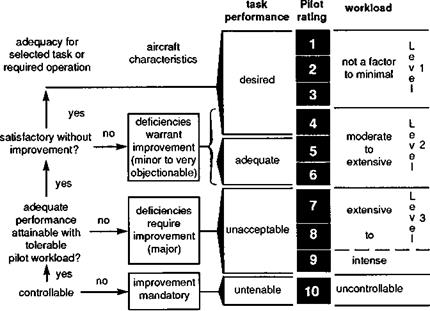
In this book we loosely divide flying qualities into two categories – handling qualities, reflecting the aircraft’s behaviour in response to pilot controls, and ride qualities, reflecting the response to external disturbances. Agreement on definitions is not widespread and we shall return to some of the debating points later in Chapter 6. A most useful definition of handling qualities has been provided by Cooper and Harper (Ref 2.30) as ‘those qualities or characteristics of an aircraft that govern the ease and precision with which a pilot is able to perform the tasks required in support of an aircraft role’. We shall expand on this definition later, but as a starting point it has stood the test of time and is in widespread use today. It is worth elaborating on the key words in this definition. Quantifying an aircraft’s characteristics or its internal attributes, while complex and selective, can be achieved on a rational and systematic basis; after all, an aircraft’s response is largely predictable and repeatable. Defining a useful task or mission is also relatively straightforward, although we have to be very careful to recognize the importance of the task performance levels required. Quantifying the pilot’s abilities is considerably more difficult and elusive. To this end, the Cooper-Harper pilot subjective rating scale (Ref. 2.30) was introduced and has now achieved almost universal acceptance as a measure of handling qualities.
|
Fig. 2.35 The Cooper – Harper handling qualities rating scale – summarized form |
Assuming that the reader has made it this far, he or she may feel somewhat daunted at the scale of the modelling task described on this Tour; if so, then Chapters 3, 4 and 5 will offer little respite, as the subject becomes even deeper and broader. If, on the other hand, the reader is motivated by this facet of flight dynamics, then the later chapters should bring further delights, as well as the tools and knowledge that are essential for practising the flight dynamics discipline. The modelling activity has been conveniently characterized in terms of frequency and amplitude; we refer back to Fig. 2.14 for setting the framework and highlight again the merging with the loads and vibration disciplines. Later chapters will discuss this overlap in greater detail, emphasizing that while there is a conceptual boundary defined by the pilot-controllable frequencies, in practice the problems actually begin to overlap at the edges of the flight envelope and where high gain active control is employed.
Much of the ground covered in this part of the Tour has utilized analytic approximations to aircraft and rotor dynamics; this approach is always required to provide physical insight and will be employed to a great extent in the later modelling chapters. The general approach will be to search among the coupled-interacting components for combinations of motion that are, in some sense, weakly coupled; if they can be found, there lies the key to analytic approximations. However, we cannot escape the complexity of both the aerodynamic and structural modelling, and Chapter 3 will formulate
expressions for the loads from first principles; analytic approximations can then be validated against the more comprehensive theories to establish their range of application. With today’s computing performance and new functionality, the approach to modelling is developing rapidly. For example, there are now far more papers published that compare numerical rather than analytic results from comprehensive models with test data. Analytic approximations tend, nowadays, to be a rarity. The comprehensive models are expected to be more accurate and have higher fidelity, but the cost is sometimes the loss of physical understanding, and the author is particularly sensitive to this, having lived through the transition from a previous era, characterized by analytic modelling, to the present, more numerical one. Chapters 3 and 4 will reflect this and will be packed full with the author’s well-established prejudices.
We have touched on the vast topic of validation and the question of how good a model has to be. This topic will be revisited in Chapter 5; the answer is actually quite simple – it depends! The author likens the question, ‘How good is your model?’ to ‘what’s the weather like on Earth?’ It depends on where you are and the time of year, etc. So while the initial, somewhat defensive answer may be simple, to address the question seriously is a major task. This book will take a snapshot of the scene in 1995, but things are moving fast in this field, and new validation criteria along with test data from individual components, all matched to more comprehensive models, are likely to change the ‘weather’ considerably within the next 5 years.
In the modelling of helicopter flight dynamics, of principal concern are the flying qualities. The last 10 years has seen extensive development of quality criteria, and the accurate prediction of the associated handling and ride qualities parameters is now at the forefront of all functional validation which conveniently leads us to the next stage of the Tour.
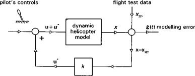
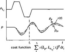
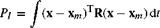
The process of validation and fidelity assessment is concerned ultimately with understanding the accuracy and range of application of the various assumptions distributed throughout the modelling. At the heart of this lies the prediction of the external forces and moments, particularly the aerodynamic loads. One of the problems with direct or forward simulation, where the simulation model is driven by prescribed control inputs and the motion time histories derived from the integration of the forces and moments, is that the comparisons of simulation and flight can very quickly depart with even the smallest modelling errors. The value of the comparison in providing validation insight then becomes very dubious, as the simulation and flight are soon engaged in very different manoeuvres. The concept behind inverse simulation is to prescribe, using flight test data, the motion of the helicopter in the simulation and hence derive the required forces and moments for comparison with those predicted by theory. One form of the process can be conceived in closed-loop form with the error between the model and flight forming the function to be minimized by a feedback controller (Fig. 2.34). If we assume that the model structure is linear with n DoFs x, for which we also have flight
|
Fig. 2.34 Inverse simulation as a feedback process |
measurements xm, then the process can be written as
The modelling errors have been embodied into a dummy control variable u* in eqns 2.80 and 2.81. The gain matrix k can be determined using a variety of minimization algorithms to achieve the optimum match between flight and theory; the example given in Ref. 2.26 uses the conventional quadratic least-squares performance index
 (2.82)
The elements of the weighting matrix R can be selected to achieve distributed fits over the different motion variables. The method is actually a special form of system identification, with the unmodelled effects being estimated as effective controls. The latter can then be converted into residual forces and moments that can be analysed to describe the unmodelled loads or DoFs. A special form of the inverse simulation method that has received greatest attention (Refs 2.27, 2.28) corresponds to the case where the feedback control in Fig. 2.34 and eqn 2.81 has infinite gain. Effectively, four of the helicopter’s DoFs can now be prescribed exactly, and the remaining DoFs and the four controls are then estimated. The technique was originally developed to provide an assessment tool for flying qualities; the kinematics of MTEs could be prescribed and the ability of different aircraft configurations to fly through the manoeuvres compared (Ref. 2.29). Later, the technique was used to support validation work and has now become fairly well established (Ref. 2.26).
How well a theoretical simulation needs to model the helicopter behaviour depends very much on the application; in the simulation world the measure of quality is described as the fidelity or validation level. Fidelity is normally judged by comparison with test data, both model and full scale. The validation process can be described in terms of two kinds of fidelity-functional and physical (Ref. 2.19), defined as follows:
|
Fig. 2.31 Nonlinear pitch response for Lynx at 100 knots |
Functional fidelity is the level of fidelity of the overall model to achieve compliance with some functional requirement, e. g., for our application, can the model be used to predict flying qualities parameters?
Physical fidelity is the level of fidelity of the individual modelling assumptions in the model components, in terms of their ability to represent the underlying physics, e. g., does the rotor aerodynamic inflow formulation capture the fluid mechanics of the wake correctly?
It is convenient and also useful to distinguish between these two approaches because they focus attention on the two ends of the problem – have we modelled the physics correctly and does the pilot perceive that the simulation ‘feels’ right? It might be imagined that the one would follow from the other and while this is true to an extent, it is also true that simulation models will continue to be characterized by a collection of aerodynamic and structural approximations, patched together and each correct over a limited range, for the foreseeable future. It is also something of a paradox that the conceptual product of complexity and physical understanding can effectively be constant in simulation. The more complex the model becomes, then while the model fidelity may be increasing, the ability to interpret cause and effect and hence gain physical understanding of the model behaviour diminishes. Against this stands the argument that, in general, only through adding complexity can fidelity be improved. A general rule of thumb is that the model needs to be only as complex as the fidelity requirements dictate; improvements beyond this are generally not cost-effective. The problem is that we typically do not know how far to go at the initial stages of a model
development, and we need to be guided by the results of validation studies reported in the literature. The last few years have seen a surge of activity in this research area, with the techniques of system identification underpinning practically all the progress (Refs 2.20-2.22). System identification is essentially a process of reconstructing a simulation model structure and associated parameters from experimental data. The techniques range from simple curve fitting to complex statistical error analysis, but have been used in aeronautics in various guises from the early days of data analysis (see the work of Shinbrot in Ref. 2.23). The helicopter presents special problems to system identification, but these are nowadays fairly well understood, if not always accounted for, and recent experience has made these techniques much more accessible to the helicopter flight dynamicist.
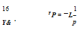
An example illustrating the essence of system identification can be drawn from the roll response dynamics described earlier in this chapter; if we assume the first-order model structure, then the equation of motion and measurement equation take the form
P — Lpp — L&ic ®lc + Ep (2 73)
P = f (Pm) + Em
The second equation is included to show that in most cases, we shall be considering problems where the variable or state of interest is not the same as that measured; there will generally be some measurement error function Em and some calibration function f involved. Also, the equation of motion will not fully model the situation and we introduce the process error function ep. Ironically, it is the estimation of the characteristics of these error or noise functions that has motivated the development of a significant amount of the system identification methodology.
The solution for roll rate can be written in either a form suitable for forward (numerical) integration
t
P = P0 + / (LpP(r) + L вс °ic (t ))dT (2.74)
0
or an analytic form
t
p — poeLpt + j eLp(t-t)Lelc91c(t)dT (2.75)
0
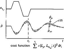
The identification problem associated with eqns 2.73 becomes, ‘from flight test measurements of roll rate response to a measured lateral cyclic input, estimate values of the damping and control sensitivity derivatives Lp and Le1c ’. In starting at this point, we are actually skipping over two of the three subprocesses of system identification – state estimation and model structure estimation, processes that aim to quantify better the measurement and process noise. There are two general approaches to solving the identification problem – equation error and output error. With the equation error method, we work with the first equation of 2.73, but we need measurements of both roll rate and roll acceleration, and rewrite the equation in the form
|
Fig. 2.32 Equation error identification process |
Subscripts m and e denote measurements and estimated states respectively. The identification process now involves achieving the best fit between the estimated roll acceleration pe from eqn 2.76 and the measured roll acceleration pm, varying the parameters Lp and Lo1c to achieve the fit (Fig. 2.32). Equation 2.76 will yield one-fit equation for each measurement point, and hence with n measurement times we have two unknowns and n equations – the classic overdetermined problem. In matrix form, the n equations can be combined in the form
x = By + e (2.77)
where x is the vector of acceleration measurements, B is the (n x 2) matrix of roll rate and lateral cyclic measurements and y is the vector of unknown derivatives L p and Lo1c; e is the error vector function. Equation 2.77 cannot be inverted in the conventional manner because the matrix B is not square. However, a pseudo-inverse can be defined that will provide the so-called least-squares solution to the fitting process, i. e., the error function is minimized so that the sum of the squares of the error between, measured and estimated acceleration is minimized over a defined time interval. The least-squares solution is given by
y = (BTB)-1BTx (2.78)
Provided that the errors are randomly distributed with a normal distribution and zero mean, the derivatives so estimated from eqn 2.78 will be unbiased and have high confidence factors.
The second approach to system identification is the output error method, where the starting equation is the solution or ‘output’ of the equation of motion. In the present example, either the analytic (eqn 2.74) or numerical (eqn 2.73) solution can be used; it is usually more convenient to work with the latter, giving the estimated roll rate in this case as
t
pe = P0m + J (Lp Pm (T) + L Ole Oicm (T ))dT (2.79)
0
|
Fig. 2.33 Output error identification process |
The error function is then formed from the difference between the measured and estimated roll rate, which can once again be minimized in a least-squares sense across the time history to yield the best estimates of the damping and control derivatives (Fig. 2.33).
Provided that the model structures are correct, the processes we have described will always yield ‘good’ derivative estimates in the absence of ‘noise’, assuming that enough measurements are available to cover the frequencies of interest; in fact, the two methods are equivalent in this simple case. Most identification work with simulated data falls into this category, and new variants of the two basic methods are often tested with simulation data prior to being applied to test data. Without contamination with a realistic level of noise, simulation data can give a very misleading impression of the robustness level of system identification methods applied to helicopters. Expanding on the above, we can classify noise into two sources for the purposes of the discussion:
(1) measurement noise, appearing on the measured signals;
(2) process noise, appearing on the response outputs, reflecting unmodelled effects.
It can be shown (Ref. 2.24, Klein) that results from equation error methods are susceptible to measurement noise, while those from output error analysis suffer from process noise. Both can go terribly wrong if the error sources are deterministic and cannot therefore be modelled as random noise. An approach that purports to account for both error sources is the so-called maximum likelihood technique, whereby the output error method is used in conjunction with a filtering process, that calculates the error functions iteratively with the model parameters.
Identifying stability and control derivatives from flight test data can be used to provide accurate linear models for control law design or in the estimation of handling qualities parameters. Our principal interest in this Tour is the application to simulation model validation. How can we use the estimated parameters to quantify the levels of modelling fidelity? The difficulty is that the estimated parameters are made up of contributions from many different elements, e. g., main rotor and empennage, and the process of isolating the source of a deficient force or moment prediction is not obvious. Two approaches to tackling this problem are described in Ref. 2.25; one where the model parameters are physically based and where the modelling element of interest is isolated from the other components through prescribed dynamics – the so-called open-loop or constrained method. The second method involves establishing the relationship between the derivatives and the physical rotorcraft parameters, hence enabling the degree of distortion of the physical parameters required to match the test data. Both these methods are useful and have been used in several different applications over the last few years.
Large parameter distortions most commonly result from one of two sources in helicopter flight dynamics, both related to model structure deficiencies – missing DoFs or missing nonlinearities, or a combination of both. A certain degree of model structure mismatch will always be present and will be reflected in the confidence values in the estimated parameters. Large errors can, however, lead to unrealistic values of some parameters that are effectively being used to compensate for the missing parts. Knowing when this is happening in a particular application is part of the ‘art’ of system identification. One of the keys to success involves designing an appropriate test input that ensures that the model structure of interest remains valid in terms of frequency and amplitude, bringing us back to the two characteristic dimensions of modelling. A relatively new technique that has considerable potential in this area is the method of inverse simulation.
Returning now to the general linear problem, we shall find it convenient to use the vector-matrix shorthand form of the equations of motion, written in the form
dx
—— Ax = Bu + f(t) (2.71)
dt
where
x = {u, w, q, 9, v, p, ф, r, ф}
A and B are the matrices of stability and control derivatives, and we have included a forcing function f(t) to represent external disturbances, e. g., gusts. Equation 2.71 is a linear differential equation with constant coefficients that has an exact solution with analytic form
t
x(t) = Y(t) x(0) + у Y(t — t ) (Bu + f(T)) dr 0
Y(t) = 0, t < 0
Y(t) = U diag[exp(kft)]U—1, t > 0 (2.72)
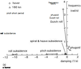
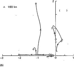
The response behaviour is uniquely determined by the principal matrix solution Y(t) (Ref. 2.18), which is itself derived from the eigenvalues kf and eigenvectors u; (arranged as columns in the matrix U) of the matrix A. The stability of small motions about the trim condition is determined by the real parts of the eigenvalues and the complete response to controls u or disturbances f is a linear combination of the eigenvectors. Figures 2.29(a) and (b) show how the eigenvalues for the Helisim Lynx and Helisim Puma configurations vary with speed from hover to 160 knots; at the higher speeds, the conventional fixed-wing parlance for naming the modes associated with the eigenvalues is appropriate. The pitch instability at high speed for the hingeless rotor Helisim Lynx has already been discussed in terms of the loss of manoeuvre stability. At lower speeds the modes change character, until at the hover they take on shapes peculiar to the helicopter, e. g., heave/yaw oscillation, pitch/roll pendulum mode. The heave/yaw mode tends to be coupled, due to the fuselage yaw reaction to changes in rotor torque, induced by perturbations in the rotor heave/inflow velocity. The eigenvectors represent the mode shapes, or the ratio of the response contributions in the various DoFs. The
![]()
 |
 damping (1 Is)
Fig. 2.29 (a) Variation of Lynx eigenvalues with forward speed; (b) variation of Puma
eigenvalues with forward speed
modes are linearly independent, meaning that no one can be made up as a collection of the others. If the initial conditions, control inputs or gust disturbance have their energy distributed throughout the DoFs with the same ratio as a particular eigenvector, then the response will be restricted to that mode only. More discussion on the physics of the modes can be found in Chapter 4.
The key value of the linearized equations of motion is in the analysis of stability; they also form the basic model for control system design. Both uses draw on the considerable range of mathematical techniques developed for linear systems analysis. We shall return to these later in Chapters 4 and 5, but we need to say a little more about the two inherently nonlinear problems of flight mechanics – trim and response.
|
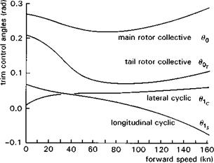
Fig. 2.30 Variation of trim control angles with forward speed for Puma |
The former is obtained as the solution to the algebraic eqn 2.2 and generally takes the form of the controls required to hold a steady flight condition. The general form of control variations with forward speed is illustrated in Fig. 2.30. The longitudinal cyclic moves forward as speed increases to counteract the flapback caused by forward speed effects (Mu effect). The lateral cyclic has to compensate for the rolling moment due to the tail rotor thrust and also the lateral flapping induced in response to coning and longitudinal variations in rotor inflow. The collective follows the shape of the power required, decreasing to the minimum power speed at around 70 knots then increasing again sharply at higher speeds. The tail rotor collective follows the general shape of the main rotor collective; at high-speed the pedal required decreases as some of the anti-torque yawing moment is typically produced by the vertical stabilizer.
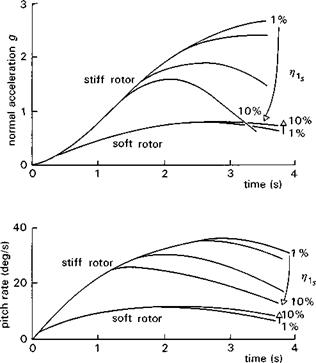
While it is true that the response problem is inherently nonlinear, it is also true that for small perturbations, the linearized equations developed for stability analysis can be used to predict the dynamic behaviour. Figure 2.31 illustrates and compares the pitch response of the Helisim Lynx fitted with a standard and soft rotor as a function of control input size; the response is normalized by the input size to indicate the degree of nonlinearity present. Also shown in the figure is the normal acceleration response; clearly, for the larger inputs the assumptions of constant speed implicit in any linearization would break down for the standard stiffer rotor. Also the rotor thrust would have changed significantly in the manoeuvre and, together with the larger speed excursions for the stiffer rotor, produce the nonlinear response shown.
The rotor thrust T in hover can be determined from the integration of the lift forces on the blades
 (2.53)
Using eqns 2.17-2.21, the thrust coefficient in hover and vertical flight can be written
as
 (2.54)
Again, we have assumed that the induced downwash ki is constant over the rotor disc; Hz is the normal velocity of the rotor, positive down and approximates to the aircraft velocity component w. Before we can calculate the vertical damping derivative Zw, we need an expression for the uniform downwash. The induced rotor downwash is one of the most important individual components of helicopter flight dynamics; it can also be the most complex. The downwash, representing the discharged energy from the lifting rotor, actually takes the form of a spiralling vortex wake with velocities that vary in space and time. We shall give a more comprehensive treatment in Chapter 3, but in this introduction to the topic we make some major simplifications. Assuming that the rotor takes the form of an actuator disc (Ref. 2.17) supporting a pressure change and accelerating the air mass, the induced velocity can be derived by equating the work done by the integrated pressures with the change in air-mass momentum. The hover downwash over the rotor disc can then be written as
 (2.55)
where Ad is the rotor disc area and p is the air density. Or, in normalized form
 (2.56)
The rotor thrust coefficient Ct will typically vary between 0.005 and 0.01 for helicopters in 1 g flight, depending on the tip speed, density altitude and aircraft weight. Hover downwash ki then varies between 0.05 and 0.07. The physical downwash is
proportional to the square root of the rotor disc loading, Ld, and at sea level is given
by
Vihover = 14-VLd (2.57)
For low disc loading rotors (Ld = 6 lb/ft2, 280N/m2), the downwash is about 35 ft/s (10 m/s); for high disc loading rotors (Ld = 12 lb/ft2, 560 N/m2), the downwash rises to over 50 ft/s (l5 m/s).
The simple momentum considerations that led to eqn 2.55 can be extended to the energy and hence power required in the hover
![]() T3/2
T3/2
Pi = T Vi = ——————-
i i V(2Md)
The subscript i refers to the induced power which accounts for about 70% of the power required in hover; for a 10000-lb (4540 kg) helicopter developing a downwash of 40 ft/s (typical of a Lynx), the induced power comes to nearly 730 HP (545 kW). Equations 2.54 and 2.56 can be used to derive the heave damping derivative
where
![]() d Ct 2a0s ki
d Ct 2a0s ki
d^z 16ki + a^s
and hence
where Ab is the blade area and s the solidity, or ratio of blade area to disc area. For our reference Helisim Lynx configuration, the value of Zw is about —0.33/s in hover, giving a heave motion time constant of about 3 s (rise time to 63% of steady state). This is typical of heave time constants for most helicopters in hover. With such a long time constant, the vertical response would seem more like an acceleration than a velocity type to the pilot. The response to vertical gusts, wg, can be derived from the first-order approximation to the heave dynamics
![]() dw
dw
![]() ——— Zww = Zww
——— Zww = Zww
dt
The initial acceleration response to a sharp-edge vertical gust provides a useful measure of the ride qualities of the helicopter, in terms of vertical bumpiness
A gust of magnitude 30 ft/s (10 m/s) would therefore produce an acceleration bump in Helisim Lynx of about 0.3 g. Additional effects such as the blade flapping, downwash lag and rotor penetration will modify the response. Vertical gusts of this magnitude
are rare in the hovering regime close to the ground, and, generally speaking, the low values of Zw and the typical gust strengths make the vertical gust response in hovering flight fairly insignificant. There are some important exceptions to this general result, e. g., helicopters operating close to structures or obstacles with large downdrafts (e. g., approaching oil rigs), that make the vertical performance and handling qualities, such as power margin and heave sensitivity, particularly critical. We shall return to gust response as a special topic in Chapter 5.
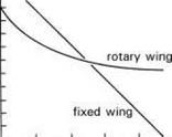
The coefficient outside the parenthesis in eqn 2.67 is the expression for the corresponding value of heave damping for a fixed-wing aircraft with wing area Aw.
The key parameter is again blade/wing loading. The factor in parenthesis in eqn 2.67 indicates that the helicopter heave damping or gust response parameter flattens off at high-speed while the fixed-wing gust sensitivity continues to increase linearly. At lower speeds, the rotary-wing factor in eqn 2.67 increases to greater than one. Typical values of lift curve slope for a helicopter blade can be as much as 50% higher than a moderate aspect-ratio aeroplane wing. It would seem therefore that all else being equal, the helicopter will be more sensitive to gusts at low-speed. In reality, typical blade loadings are considerably higher than wing loadings for the same aircraft weight; values of 100 lb/ft2 (4800 N/m2) are typical for helicopters, while fixed-wing executive transports have wing loadings around 40 lb/ft2 (1900 N/m2). Military jets have higher wing loadings, up to 70 lb/ft2 (3350 N/m2) for an aircraft like the Harrier, but this is still quite a bit lower than typical blade loadings. Figure 2.28 shows a comparison of heave damping for our Helisim Puma helicopter (a0 = 6, blade area = 144 ft2 (13.4 m2)) with a similar class of fixed-wing transport (a0 = 4, wing area = 350 ft2 (32.6 m2)), both weighing in at 13 500 lb (6130 kg). Only the curve for the rotary-wing aircraft has been extended to zero speed, the Puma point corresponding to the value
![]()
|
|
|
|
|
|
|
|
|
|
|
|
|
|
|
![]()
of Zw given by eqn 2.61. The helicopter is seen to be more sensitive to gusts below about 50 m/s (150 ft/s); above this speed, the helicopter value remains constant, while the aeroplane response continues to increase. Three points are worth developing about this result for the helicopter:
(1) The alleviation due to blade flapping is often cited as a major cause of the lower gust sensitivity of helicopters. In fact, this effect is fairly insignificant as far as the vertical gust response is concerned. The rotor coning response, which determines the way that the vertical load is transmitted to the fuselage, reaches its steady state very quickly, typically in about 100 ms. While this delay will take the edge off a truly sharp gust, in reality, the gust front is usually of ramp form, extending over several of the blade response time constants.
(2) The Zw derivative reflects the initial response only; a full assessment of ride qualities will need to take into account the short-term transient response of the helicopter and, of course, the shape of the gust. We shall see later in Chapter 5 that there is a key relationship between gust shape and aircraft short-term response that leads to the concept of the worst case gust, when there is ‘tuning’ or ‘resonance’ between the aircraft response and the gust scale/amplitude.
(3)
The third point concerns the insensitivity of the response with speed for the helicopter at higher speeds. It is not obvious why this should be the case, but the result is clearly connected with the rotation of the rotor. To explore this point further, it will help to revisit the thrust equation, thus exploiting the modelling approach to the full:
where
Ut ~ r + д sin ф, Up = ptz — k; — дв cos ф — rв (2.70)
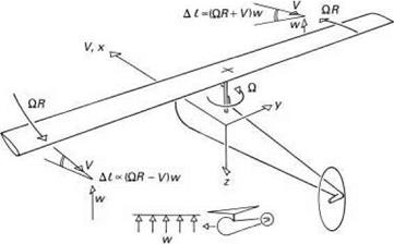
The vertical gust response stems from the product of velocities Up Ut in eqn 2.69. It can be seen from eqn 2.70 that the forward velocity term in Ut varies one-per-rev, therefore contributing nothing to the quasi-steady hub loading. The most significant contribution to the gust response in the fuselage comes through as an N – per-rev vibration superimposed on the steady component represented by the derivative Zw. The ride bumpiness of a helicopter therefore has quite a different character from that of a fixed-wing aircraft where the lift component proportional to velocity dominates the response.
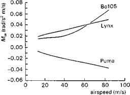
In simple physical terms the derivative Mw represents the change in pitching moment about the aircraft’s centre of mass when the aircraft is subjected to a perturbation in normal velocity w or, effectively, incidence. If the perturbation leads to a positive, pitch-up, moment, then Mw is positive and the aircraft is said to be statically unstable in pitch; if Mw is negative then the aircraft is statically stable. Static stability refers to the initial tendency only and the Mw effect is analogous to the spring in a simple spring/mass/damper dynamic system. In fixed-wing aircraft flight dynamics, the derivative is proportional to the distance between the aircraft’s centre of mass and the overall aerodynamic centre, i. e., the point about which the resultant lift force acts when the incidence is changed. This distance metric, in normalized form referred to as the static margin, does not carry directly across to helicopters, because as the incidence changes, not only does the aerodynamic lift on the rotor change, but it also rotates (as the rotor disc tilts). So, while we can consider an effective stafic margin for helicopters, this is not commonly used because the parameter is very configuration dependent and is also a function of perturbation amplitude. There is another reason why the static margin concept has not been adopted in helicopter flight dynamics. Prior to the deliberate design of fixed-wing aircraft with negative static margins to improve performance, fundamental configuration and layout parameters were defined to achieve a positive static margin. Most helicopters are inherently unstable in pitch and very little can be achieved with layout and configuration parameters to change this, other than through the stabilizing effect of a large tailplane at high-speed (e. g., UH-60). When the rotor is subjected to a positive incidence change in forward flight, the advancing blade experiences a greater lift increment than does the retreating blade (see Fig. 2.25). The 90° phase shift in response means that the rotor disc flaps back and cones up and hence applies a positive pitching moment to the aircraft. The rotor contribution to Mw will tend to increase with forward speed; the contributions from the fuselage and horizontal stabilizer will also increase with airspeed but tend to cancel each other, leaving the rotor contribution as the primary contribution. Figure 2.26 illustrates the variation in Mw for the three baseline aircraft in forward flight. The effect of the hingeless rotors on Mw is quite striking, leading to large destabilizing moments at high speed. It is
|
Fig. 2.25 Incidence perturbation on advancing and retreating blades during encounter with vertical gust |
|
Fig. 2.26 Variation of static stability derivative, Mw, with forward speed for Bo105, Lynx and Puma |
interesting to consider the effect of this static instability on the dynamic, or longer term, stability of the aircraft.
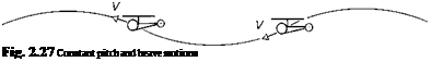
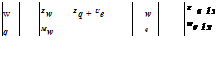
A standard approximation to the short-term dynamic response of a fixed-wing aircraft can be derived by considering the coupled pitch/heave motions, assuming that the airspeed is constant. This is a gross approximation for helicopters but can be used to approximate high-speed flight in certain circumstances (Ref. 2.16). Figure 2.27 illustrates generalized longitudinal motion, distinguishing between pitch and incidence. For the present, we postulate that the assumption of constant speed applies, and that the perturbations in heave velocity w, and pitch rate q, can be described by the linearized equations:
Iyyq — 5 M
|
 |
constant incidence a varying pitch в
constant pitch в varying incidence a
 |
||||
where Iyy is the pitch moment of inertia of the helicopter about the reference axes and Ma is the mass. Ue is the trim or equilibrium forward velocity and b Z and b M are the perturbation Z force and pitching moment. Expanding the perturbed force and moment into derivative form, we can write the perturbation equations of motion in matrix form:
The derivatives Zw, Mq, etc., correspond to the linear terms in the expansion of the normal force and pitch moment, as described in eqn 2.45. It is more convenient to discuss these derivatives in semi-normalized form, and we therefore write these in eqn 2.50, and throughout the book, without any distinguishing dressings, as
The solution to eqn 2.50 is given by a combination of transient and steady-state components, the former having an exponential character, with the exponents, the stability discriminants, as the solutions to the characteristic equation
Л2 — (Zw + Mq)X + Zw Mq — Mw (Zq + Ue) — 0 (2.52)
According to eqn 2.52, when the static stability derivative Mw is zero, then the pitch and heave motions are uncoupled giving two first-order transients (decay rates given by Zw and Mq). As Mw becomes increasingly positive, the aircraft will not experience dynamic instability until the manoeuvre margin, the stiffness term in eqn 2.52, becomes zero. Long before this however, the above approximation breaks down.
One of the chief reasons why this short period approximation has a limited application range with helicopters is the strong coupling with speed variations, reflected in the speed derivatives, particularly Mu . This speed stability derivative is normally zero for fixed-wing aircraft at subsonic speeds, on account of the moments from all aerodynamic surfaces being proportional to dynamic pressure and hence perturbations tend to cancel one another. For the helicopter, the derivative Mu is significant even in the hover, again caused by differential effects on advancing and retreating blades leading to flapback; so while this positive derivative can be described as statically stable, it
actually contributes to the dynamic instability of the pitch phugoid. This effect will be further explored in Chapter 4, along with the second reason why low-order approximations are less widely applicable for helicopters, namely cross-coupling. Practically all helicopter motions are coupled, but some couplings are more significant than others, in terms of their effect on the direct response on the one hand, and the degree of pilot off-axis compensation required, on the other.
Alongside the fundamentals of flapping, the rotor thrust and torque response to normal velocity changes are key rotor aeromechanics effects that need some attention on this Tour.
This Tour would be incomplete without a short discussion on ‘stability and control derivatives’ and a description of typical helicopter stability characteristics. To do this we need to introduce the helicopter model configurations we shall be working with in this book and some basic principles of building the aircraft equations of motion. The three baseline simulation configurations are described in Appendix 4B and represent the Aerospatiale (ECF) SA330 Puma, Westland Lynx and MBB (ECD) Bo105 helicopters. The Puma is a transport helicopter in the 6-ton class, the Lynx is a utility transport/anti-armour helicopter in the 4-ton class and the Bo105 is a light utility/anti – armour helicopter in the 2.5-ton class. Both the Puma and Bo105 operate in civil and military variants throughout the world; the military Lynx operates with both land and sea forces throughout the world. All three helicopters were designed in the 1960s and have been continuously improved in a series of new Marks since that time. The Bo105 and Lynx were the first hingeless rotor helicopters to enter production and service. On these aircraft, both flap and lead-lag blade motion are achieved through elastic bending, with blade pitch varied through rotations at a bearing near the blade root. On the Puma, the blade flap and lead-lag motions largely occur through articulation with the hinges close to the hub centre. The distance of the hinges from the hub centre is a critical parameter in determining the magnitude of the hub moment induced by blade flapping and lagging; the moments are approximately proportional to the hinge offset, up to values of about 10% of the blade radius. Typical values of the flap hinge offset are found between 3 and 5% of the blade radius. Hingeless rotors are often quoted as having an effective hinge offset, to describe their moment-producing capability, compared with articulated rotor helicopters. The Puma has a flap hinge offset of 3.8%, while the Lynx and Bo105 have effective offsets of about 12.5 and 14% respectively. We can expect the moment capability of the two hingeless rotor aircraft to be about three times
that of the Puma. This translates into higher values of kp and Sp, and hence higher rotor moment derivatives with respect to all variables, not only rates and controls as described in the above analysis.
The simulation model of the three aircraft will be described in Chapter 3 and is based on the DRA Helisim model (Ref. 2.15). The model is generic in form, with two input files, one describing the aircraft configuration data (e. g., geometry, mass properties, aerodynamic and structural characteristics, control system parameters), the other the flight condition parameters (e. g., airspeed, climb/descentrate, sideslip and turn rate) and atmospheric conditions. The datasets for the three Helisim aircraft are located in Chapter 4, Section 4B.1, while Section 4B.2 contains charts of the stability and control derivatives. The derivatives are computed using a numerical perturbation technique applied to the full nonlinear equations of motion and are not generally derived in explicit analytic form. Chapters 3 and 4 will include some analytic formulations to illustrate the physics at work; it should be possible to gain insight into the primary aerodynamic effects for all the important derivatives in this way. The static stability derivative Mw is a good example and allows us to highlight some of the differences between fixed – and rotary-wing aircraft.
The assumptions made to establish the above approximate results have not been discussed; we have neglected detailed blade aerodynamic and deformation effects and we have assumed the rotorspeed to be constant; these are important effects that will need to be considered later in Chapter 3, but would have detracted from the main points we have tried to establish in the foregoing analysis. One of these is the concept of the motion derivative, or partial change in the rotor forces and moments with rotor motion. If the rotor were an entirely linear system, then the total force and moment could be formulated as the sum of individual effects each written as a derivative times a motion.
![]()
This approach, which will normally be valid for small enough motion, has been established in both fixed – and rotary-wing flight dynamics since the early days of flying (Ref. 2.13) and enables the stability characteristics of an aircraft to be determined. The assumption is made that the aerodynamic forces and moments can be expressed as a multi-dimensional analytic function of the motion of the aircraft about the trim condition; hence the rolling moment, for example, can be written as
![]() + terms due to higher motion derivatives (e. g., p) and controls
+ terms due to higher motion derivatives (e. g., p) and controls
For small motions, the linear terms will normally dominate and the approximation can be written in the form
L — Ltrim + Luu + Lvv + Lww + Lpp + Lqq + Lrr
+ acceleration and control terms (2.46)
In this 6 DoF approximation, each component of the helicopter will contribute to each derivative; hence, for example, there will be an Xu and an Np for the rotor, fuselage, empennage and even the tail rotor, although many of these components, while dominating some derivatives, will have a negligible contribution to others. Dynamic
effects beyond the motion in the six rigid-body DoFs will be folded into the latter in quasi-steady form, e. g., rotor, air mass dynamics and engine/transmission. For example, if the rotor DoFs were represented by the vector xr and the fuselage by xr, then the linearized, coupled equations can be written in the form
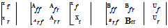 (2.47)
We have included, for completeness, fuselage and rotor controls. Folding the rotor DoFs into the fuselage as quasi-steady motions will be valid if the characteristic frequencies of the two elements are widely separate and the resultant approximation for the fuselage motion can then be written as
xf — ^Aff — AfrArr Af j xf = — AfrA-r Bf] uf + [Bfr — AfrA— Brr] Ur
(2.48)
In the above, we have employed the weakly coupled approximation theory of Milne (Ref. 2.14), an approach used extensively in Chapters 4 and 5. The technique will serve us well in reducing and hence isolating the dynamics to single DoFs in some cases, hence maximizing the potential physical insight gained from such analysis. The real strength in linearization comes from the ability to derive stability properties of the dynamic motions.
From the above discussion, we can see the importance of the two key parameters, kp and у, in determining the flapping behaviour and hence hub moment. The hub moments due to the out-of-plane rotor loads are proportional to the rotor stiffness, as given by eqns 2.14 and 2.15; these can be written in the form
Pitchmoment: M = — Nb—bp1c = —b®2^kp — 1^ вс (2.33)
Rollmoment: L = – Nb—в-в^ = —bq}Ip — 1^ f5s (2.34)
To this point in the analysis we have described rotor motions with fixed or prescribed shaft rotations to bring out the partial effects of control effectiveness and flap damping. We can now extend the analysis to shaft-free motion. To simplify the analysis we consider only the roll motion and assume that the centre of mass of the rotor and shaft lies at the hub centre. The motion of the shaft is described by the simple equation relating the rate of change of angular momentum to the applied moment:
Ixxp = L (2.35)
where Ixx is the roll moment of inertia of the helicopter. By combining eqn 2.27 with eqn 2.34, the equation describing the 1 DoF roll motion of the helicopter, with quasi-steady rotor, can be written in the first-order differential form of a rate response type:
![]() P — Lpp = L01c 01c
P — Lpp = L01c 01c
where the rolling moment ‘derivatives’ are given by
where the approximation that Sв << 1 has been made. Non-dimensionalizing by the roll moment of inertia Ixx transforms these into angular acceleration derivatives.
These are the most primitive forms of the roll damping and cyclic control derivatives for a helicopter, but they contain most of the first-order effects, as will be observed later in Chapters 4 and 5. The solution to eqn 2.36 is a simple exponential transient
|
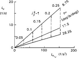
Fig. 2.22 Linear variation of rotor damping with control sensitivity in hover |
superimposed on the steady state solution. For a simple step input in lateral cyclic, this takes the form
p = -(l – eLPt)0lc (2.38)
LP
The time constant (time to reach 63% of steady state) of the motion, Tp, is given by —(1/Lp), the control sensitivity (initial acceleration) by L$1c and the rate sensitivity (steady-state rate response per degree of cyclic) by
Pss (deg/(s deg)) = —-^ = —^ (2.39)
L p 16
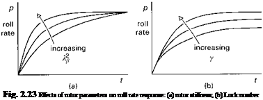
These are the three handling qualities parameters associated with the time response of eqn 2.36, and Fig. 2.22 illustrates the effects of the primary rotor parameters. The fixed parameters for this test case are Й = 35 rad/s, Nb = 4, Ip/Ixx = 0.25.
Four points are worth highlighting:
(1) contrary to ‘popular’ understanding, the steady-state roll rate response to a step lateral cyclic is independent of rotor flapping stiffness; teetering and hingeless rotors have effectively the same rate sensitivity;
(2) the rate sensitivity varies linearly with Lock number;
(3) both control sensitivity and damping increase linearly with rotor stiffness;
(4) the response time constant is inversely proportional to rotor stiffness.
These points are further brought out in the generalized sketches in Figs 2.23(a) and (b), illustrating the first-order time response in roll rate from a step lateral cyclic input. These time response characteristics were used to describe short-term handling qualities until the early 1980s when the revision to Mil Spec 8501A (Ref. 2.2) introduced the frequency domain as a more meaningful format, at least for non-classical short-term response. One of the reasons for this is that the approximation of quasi-steady flapping motion begins to break down when the separation between the frequency of rotor flap modes and fuselage attitude modes decreases. The full derivation of the equations of flap motion will be covered in Chapter 3, but to complete this analysis of rotor/fuselage
 |
coupling in hover, we shall briefly examine the next, improved, level of approximation. Equations 2.40 and 2.41 describe the coupled motion when only first-order lateral flapping (the so-called flap regressive mode) and fuselage roll are considered. The other rotor modes – the coning and advancing flap mode – and coupling into pitch, are neglected at this stage.
|
л As 01c 01s +—————— = p + |
(2.40) |
|
T01s T01s |
|
|
О II i |
(2.41) |
where
and
 (2.43)
The time constants xp1s and Tp are associated with the disc and fuselage (shaft) response respectively. The modes of motion are now coupled roll/flap with eigenvalues given by the characteristic equation
к2 + — к + = 0 (2.44)
TPu TPu Tp
The roots of eqn 2.44 can be approximated by the ‘uncoupled’ values only for small values of stiffness and relatively high values of Lock number. Figure 2.24 shows the variation of the exact and uncoupled approximate roots with (к2в — 1) for the case when Y = 8. The approximation of quasi-steady rotor behaviour will be valid for small offset articulated rotors and soft bearingless designs, but for hingeless rotors with к^ much above 1.1, the fuselage response is fast enough to be influenced by the rotor transient response, and the resultant motion is a coupled roll/flap oscillation. Note again that the rotor disc time constant is independent of stiffness and is a function only of rotorspeed and Lock number (eqn 2.43).