Category HELICOPTER FLIGHT DYNAMICS

A fundamental result of rotor dynamics emerges from the above analysis, that the flapping response is approximately 90° out of phase with the applied cyclic pitch, i. e., 01s gives в1С, and $1C gives ^1s. For blades freely articulated at the centre of rotation, or teetering rotors, the response is lagged by exactly 90° in hover; for hingeless rotors,

-2 ——- 1—1—- 1 1—i. I i.—і————– 1—j

0.0 0.2 0.4 0.6 0.Є 1.0

(C) – tli’-!-.–

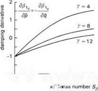
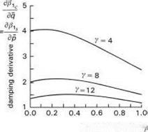
Fig. 2.21 Variation of flap derivatives with Stiffness number in hover: (a) control;
(b) damping; (c) cross-coupling

such as the Lynx and Bo105, the phase angle is about 75-80°. The phase delay is a result of the rotor being aerodynamically forced, through cyclic pitch, close to resonance, i. e., one-per-rev. The second-order character of eqn 2.22 results in a low-frequency response in-phase with inputs and a high-frequency response with a 180° phase lag. The innovation of cyclic pitch, forcing the rotor close to its natural flapping frequency, is amazingly simple and effective – practically no energy is required and a degree of pitch results in a degree of flapping. A degree of flapping can generate between 0 (for teetering rotors), 500 (for articulated rotors) and greater than 2000 N m (for hingeless rotors) of hub moment, depending on the rotor stiffness.

The flap damping derivatives, given by eqns 2.31 and 2.32, are illustrated in Figs 2.21(b) and (c). The direct flap damping, двіс/дq, is practically independent of stiffness up to Sp = 0.5; the cross-damping, д^1с/дp, varies linearly with Sp and actually changes sign at high values of Sp. In contrast with the in vacuo case, the direct flapping response now opposes the shaft motion. The disc follows the rotating shaft, lagged by an angle given by the ratio of the flap derivatives in the figures. For very heavy blades (e. g., y = 4), the direct flap response is about four times the coupled motion; for very light blades, the disc tilt angles are more equal. This rather complex response stems from the two components on the right-hand side of the flapping equation, eqn 2.22, one aerodynamic due to the distribution of airloads from the angular motion, the other
from the gyroscopic flapping motion. The resultant effect of these competing forces on the helicopter motion is also complex and needs to be revisited for further discussion in Chapters 3 and 4. Nevertheless, it should be clear to the reader that the calculation of the correct Lock number for a rotor is critical to the accurate prediction of both primary and coupled responses. Complicating factors are that most blades have strongly non­uniform mass distributions and aerodynamic loadings and any blade deformation will further effect the ratio of aerodynamic to inertia forces. The concept of the equivalent Lock number is often used in helicopter flight dynamics to encapsulate a number of these effects. The degree to which this approach is valid will be discussed later in Chapter 3.

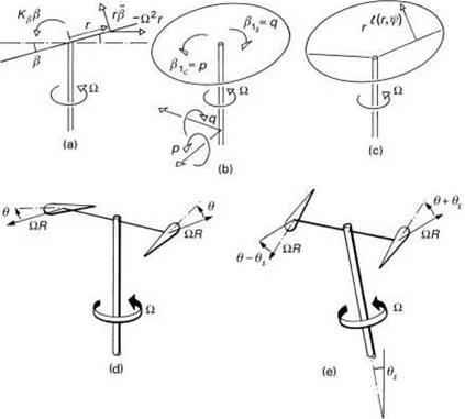
Figure 2.18(c) shows the blade in air, with the distributed aerodynamic lift t(r, ty) acting normal to the resultant velocity; we are neglecting the drag forces in this case. If the shaft is now tilted to a new reference position, the blades will realign with the shaft, even with zero spring stiffness. Figures 2.18(d) and (e) illustrate what happens. When the shaft is tilted, say, in pitch by angle 0s, the blades experience an effective cyclic pitch change with maximum and minimum at the lateral positions (ty = 90° and 180°). The blades will then flap to restore the zero hub moment condition.

For small flap angles, the equation of flap motion can now be written in the approximate form

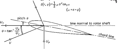A simple expression for the aerodynamic loading can be formulated with reference to Fig. 2.19, with the assumptions of two-dimensional, steady aerofoil theory, i. e.,

where V is the resultant velocity of the airflow, p the air density and c the blade chord. The lift is assumed to be proportional to the incidence of the airflow to the chord line, a, up to stalling incidence, with lift curve slope a0. In Fig. 2.19 the incidence is shown to comprise two components, one from the applied blade pitch angle 9 and one from the induced inflow ф, given by

where Ut and Up are the in-plane and normal velocity components respectively (the bar signifies non-dimensionalization with aR). Using the simplification that Up ^ Ut, eqn 2.16 can be written as

where r = r/ R and the Lock number, y, is defined as (Ref. 2.12)

The Lock number is an important non-dimensional scaling coefficient, giving the ratio of aerodynamic to inertia forces acting on a rotor blade.

To develop the present analysis further, we consider the hovering rotor and a constant inflow velocity vi over the rotor disc, so that the velocities at station r along the blade are given by

where Oq is the collective pitch and 0s and 0c the longitudinal and lateral cyclic pitch respectively. The forcing function on the right-hand side of eqn 2.22 is therefore made up of constant and first harmonic terms. In the general flight case, with the pilot active on his controls, the rotor controls Oq, 0c and 0s and the fuselage rates p and q will vary continuously with time. As a first approximation we shall assume that these variations are slow compared with the rotor blade transient flapping. We can quantify this approximation by noting that the aerodynamic damping in eqn 2.22, Y/8, varies between about 0.7 and 1.3. In terms of the response to a step input, this corresponds to rise times (to 63% of steady-state flapping) between 60 and 112° azimuth (фб3% = 16 ln(2)/Y). Rotorspeeds vary from about 27 rad/s on the AS330 Puma to about 44 rad/s on the MBB Bo105, giving flap time constants between 0.02 and 0.07 s at the extremes. Provided that the time constants associated with the control activity and fuselage angular motion are an order of magnitude greater than this, the assumption of rotor quasi-steadiness during aircraft motions will be valid. We shall return to this assumption a little later on this Tour, but, for now, we assume that the rotor flapping has time to achieve a new steady-state, one-per-rev motion following each incremental change in control and fuselage angular velocity. We write the rotor flapping motion in the quasi-steady-state form

в = во + в1с cos ф + e1s sin ф (2.24)

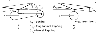
во is the rotor coning and в1с and въ the longitudinal and lateral flapping respec­tively. The cyclic flapping can be interpreted as a tilt of the rotor disc in the longitu­dinal (forward) в1с and lateral (port) вls planes. The coning has an obvious physical interpretation (see Fig. 2.20).

The quasi-steady coning and first harmonic flapping solution to eqn 2.22 can be obtained by substituting eqns 2.23 and 2.24 into eqn 2.22 and equating constant and first harmonic coefficients. Collecting terms, we can write

The partial derivatives in eqns 2.29-2.32 represent the changes in flapping with changes in cyclic pitch and shaft rotation and are shown plotted against Stiffness number for different values of y in Figs 2.21(a)-(c). Although Sp is shown plotted up to unity, a maximum realistic value for current hingeless rotors with heavy blades (small value of Y) is about 0.5, with more typical values between 0.05 and 0.3. The control derivatives illustrated in Fig. 2.21(a) show that the direct flapping response, 3^1c/991s, is approx­imately unity up to typical maximum values of stiffness, i. e., a hingeless rotor blade flaps by about the same amount as a teetering or articulated rotor. However, the varia­tion of the coupled flap response, 3P1c/’391s, is much more significant, being as much as 30% of the primary response at an Sp of 0.3. When this level of flap cross-coupling is transmitted through the hub to the fuselage, an even larger ratio of pitch/roll response coupling can result due the relative magnitudes of the aircraft inertias.

The equations of motion of a flapping rotor will be developed in a series of steps (Figs 2.18(a)-(e)), designed to highlight a number of key features of rotor behaviour. Figure 2.18(a) shows a rotating blade (Й, rad/s) free to flap (в, rad) about a hinge at the centre of rotation; to add some generality we shall add a flapping spring at the hinge (Kp, N m/rad). The flapping angle в is referred to the rotor shaft; other reference systems, e. g., relative to the control axis, are discussed in Appendix 3A. It will be shown later in Chapter 3 that this simple centre-spring representation is quite adequate for describing the flapping behaviour of teetering, articulated and hingeless or bearingless rotors, under a wide range of conditions. Initially, we consider the case of flapping in a vacuum, i. e., no aerodynamics, and we neglect the effects of gravity. The first qualitative point to grasp concerns what happens to the rotor when the rotor shaft is suddenly tilted to a new angle. For the case of the zero spring stiffness, the rotor disc

will remain aligned in its original position, there being no mechanism to generate a turning moment on the blade. With a spring added, the blade will develop a persistent oscillation about the new shaft orientation, with the inertial moment due to out-of-plane flapping and the centrifugal moment continually in balance.

The dynamic equation of flapping can be derived by taking moments about the flap hinge during accelerated motion, so that the hinge moment Kpp is balanced by the inertial moments, thus

R

Kpp = —j rm(r) [rp + rO2p} dr (2.5)

0

where m(r) is the blade mass distribution (kg/m) and (•) indicates differentiation with respect to time t. Setting О as differentiation with respect to ф = Ot, the blade azimuth angle, eqn 2.5 can be rearranged and written as

P" + Xpp = 0 (2.6)

where the flapping frequency ratio X p is given by the expression

and where the flap moment of inertia is

R

m (r ) r 2 dr

0

The two inertial terms in eqn 2.5 represent the contributions from accelerated flapping out of the plane of rotation, rp, and the in-plane centrifugal acceleration arising from the blade displacement acting towards the centre of the axis of rotation, r O2 p. Here, as will be the case throughout this book, we make the assumption that p is small, so that sin p ~ p and cos p ~ 1.

For the special case where Kp = 0, the solution to eqn 2.6 is simple harmonic motion with a natural frequency of one-per-rev, i. e., Xp = 1. If the blade is disturbed in flap, the motion will take the form of a persistent, undamped, oscillation with frequency О; the disc cut by the blade in space will take up a new tilt angle equal to the angle of the initial disturbance. Again, with Kp set to zero, there will be no tendency for the shaft to tilt in response to the flapping, since no moments can be transmitted through the flapping hinge. For the case with non-zero Kp, the frequency ratio is greater than unity and the natural frequency of disturbed motion is faster than one-per-rev, disturbed flapping taking the form of a disc precessing against the rotor rotation, if the shaft is fixed. With the shaft free to rotate, the hub moment generated by the spring will cause the shaft to rotate into the direction normal to the disc. Typically, the stiffness of a hingeless rotor blade can be represented by a spring giving an equivalent Xp of between 1.1 and 1.3. The higher values are typical of the first generation of hingeless rotor helicopters, e. g., Lynx andBo105, the lower more typical of modern bearingless designs. The overall stiffness is therefore dominated by the centrifugal force field.

Before including the effects of blade aerodynamics, we consider the case where the shaft is rotated in pitch and roll, p and q (see Fig. 2.18(b)). The blade now expe­riences additional gyroscopic accelerations caused by mutually perpendicular angular velocities, p, q and —. If we neglect the small effects of shaft angular accelerations, the equation of motion can be written as

„2 2

в + kpP = — (p cos ф — q sin ф) (2.9)

The conventional zero reference for blade azimuth is at the rear of the disc and ф is positive in the direction of rotor rotation; in eqn 2.9 the rotor is rotating anticlockwise when viewed from above. For clockwise rotors, the roll rate term would be negative. The steady-state solution to the ‘forced’ motion takes the form

в = віс cos ф + Pis sin ф (2.10)

where

These solutions represent the classic gyroscopic motions experienced when any rotating mass is rotated out of plane; the resulting motion is orthogonal to the applied rotation. в1с is a longitudinal disc tilt in response to a roll rate; P1s a lateral tilt in response to a pitch rate. The moment transmitted by the single blade to the shaft, in the rotating axes system, is simply KpP; in the non-rotating shaft axes, the moment can be written as pitch (positive nose up) and roll (positive to starboard) components

KP

M = — KpP (cos ф) = —j-(P1c(1 + cos 2ф) + P1s sin 2ф) (2.12)

Kp

L = —Kp p (sin ф) = —— (P1s (1 — cos 2ф) + P1c sin 2ф) (2.13)

Each component therefore has a steady value plus an equally large wobble at two – per-rev. For a rotor with Nb evenly spaced blades, it can be shown that the oscillatory moments cancel, leaving the steady values

This is a general result that will carry through to the situation when the rotor is working in air, i. e., the zeroth harmonic hub moments that displace the flight path of the aircraft are proportional to the tilt of the rotor disc. It is appropriate to highlight that we have neglected the moment of the in-plane rotor loads in forming these hub moment expressions. They are therefore strictly approximations to a more complex effect, which we shall discuss in more detail in Chapter 3. We shall see, however, that the aerodynamic loads are not only one-per-rev, but also two and higher, giving rise to vibratory moments. Before considering the effects of aerodynamics, there are two

points that need to be made about the solution given by eqn 2.11. First, what happens when Xp = 1? This is the classic case of resonance, when according to theory, the response becomes infinite; clearly, the assumption of small flap angles would break down well before this and the nonlinearity in the centrifugal stiffening with amplitude would limit the motion. The second point is that the solution given by eqn 2.11 is only part of the complete solution. Unless the initial conditions of the blade motion were very carefully set up, the response would actually be the sum of two undamped motions, one with the one-per-rev forcing frequency, and the other with the natural frequency Xв. A complex response would develop, with the combination of two close frequencies leading to a beating response or, in special cases, non-periodic ‘chaotic’ behaviour. Such situations are somewhat academic for the helicopter, as the aerodynamic forces distort the response described above in a dramatic way.

Continuing the discussion of the 6 DoF model, the solutions to the three fundamental problems of flight dynamics can be written as

The trim solution is represented by the zero of a nonlinear algebraic function, where the controls ue required to hold a defined state xe (subscript e refers to equilibrium) are computed. With four controls, only four states can be prescribed in trim, the remaining set forming into the additional unknowns in eqn 2.1. A trimmed flight condition is defined as one in which the rate of change (of magnitude) of the aircraft’s state vector is zero and the resultant of the applied forces and moments is zero. In a trimmed manoeuvre, the aircraft will be accelerating under the action of non-zero resultant aerodynamic and gravitational forces and moments, but these will then be balanced by effects such as centrifugal and gyroscopic inertial forces and moments. The trim equations and associated problems, e. g., predicting performance and control margins, will be further developed in Chapter 4.

The solution of the stability problem is found by linearizing the equations about a particular trim condition and computing the eigenvalues of the aircraft system matrix,

written in eqn 2.3 as the partial derivative of the forcing vector with respect to the system states. After linearization of eqn 2.1, the resulting first-order, constant coef­ficient differential equations have solutions of the form ekt, the stability of which is determined by the signs of the real parts of the eigenvalues k. The stability thus found refers to small motions about the trim point; will the aircraft return to – or depart from – the trim point if disturbed by, say, a gust? For larger motions, nonlinearities can alter the behaviour and recourse to the full equations is usually necessary.

The response solution given by eqn 2.4 is found from the time integral of the forc­ing function and allows the evolution of the aircraft states, forces and moments to be computed following disturbed initial conditions x(0), and/or prescribed control inputs and atmospheric disturbances. The nonlinear equations are usually solved numerically; analytical solutions generally do not exist. Sometimes, narrow-range approximate so­lutions can be found to describe special large-amplitude nonlinear motion, e. g., limit cycles, but these are exceptional and usually developed to support the diagnosis of behaviour unaccounted for in the original design.

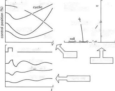
The sketches in Fig. 2.17 illustrate typical ways in which trim, stability and re­sponse results are presented; the key variable in the trim and stability sketches is the helicopter’s forward speed. The trim control positions are shown with their character­istic shapes; the stability characteristics are shown as loci of eigenvalues plotted on the complex plane; the short-term responses to step inputs, or the step responses, are shown as a function of time. This form of presentation will be revisited later on this Tour and in later chapters.

The reader of this Tour may feel too quickly plunged into abstraction with the above equations and their descriptions; the intention is to give some exposure to math­ematical concepts which are part of the toolkit of the flight dynamicist. Fluency in the

short! period /

spiral ft (1/s)

STABILITY

pitch rate

FIFSPQNSE

parlance of this mathematics is essential for the serious practitioner. Perhaps even more essential is a thorough understanding of the fundamentals of rotor flapping behaviour, which is the next stop on this Tour; here we shall need to rely extensively on theoretical analysis. A full derivation of the results will be given later in Chapters 3, 4 and 5.

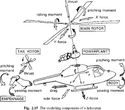
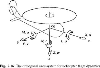
The behaviour of a helicopter in flight can be modelled as the combination of a large number of interacting subsystems. Figure 2.15 highlights the main rotor element, the fuselage, powerplant, flight control system, empennage and tail rotor elements and the resulting forces and moments. Shown in simplified form in Fig. 2.16 is the orthogonal body axes system, fixed at the centre of gravity/mass (cg/cm) of the whole aircraft, about which the aircraft dynamics are referred. Strictly speaking, the cg will move as the rotor blades flap, but we shall assume that the cg is located at the mean position, relative to a particular trim state. The equations governing the behaviour of these interactions are developed from the application of physical laws, e. g., conservation of energy and Newton’s laws of motion, to the individual components, and commonly take the form of nonlinear differential equations written in the first-order vector form

dx

-= f (X, u, t) (2.1)

dt

with initial conditions x(0) = xo.

x (t) is the column vector of state variables; u (t) is the vector of control variables and f is a nonlinear function of the aircraft motion, control inputs and external distur­bances. The reader is directed to Appendix 4A for a brief exposition on the matrix – vector theory used in this and later chapters. For the special case where only the six rigid-body degrees of freedom (DoFs) are considered, the state vector x comprises the three translational velocity components u, v and w, the three rotational velocity components p, q and r and the Euler angles ф, 9 and ф. The three Euler attitude an­gles augment the equations of motion through the kinematic relationship between the

fuselage rates p, q and r and the rates of change of the Euler angles. The velocities are referred to an axes system fixed at the cg as shown in Fig. 2.16 and the Euler angles define the orientation of the fuselage with respect to an earth fixed axes system.

The DoFs are usually arranged in the state vector as longitudinal and lateral motion subsets, as

x = {u, w, q, 9, v, p, ф, r, ф}

The function f then contains the applied forces and moments, again referred to the aircraft cg, from aerodynamic, structural, gravitational and inertial sources. Strictly speaking, the inertial and gravitational forces are not ‘applied’, but it is convenient to label them so and place them on the right-hand side of the describing equation. The derivation of these equations from Newton’s laws of motion will be carried out later in Chapter 3 and its appendix. It is important to note that this six DoF model, while itself complex and widely used, is still an approximation to the aircraft be­haviour; all higher DoFs, associated with the rotors (including aeroelastic effects), powerplant/transmission, control system and the disturbed airflow, are embodied in a quasi-steady manner in the equations, having lost their own individual dynamics and independence as DoFs in the model reduction. This process of approximation is a common feature of flight dynamics, in the search for simplicity to enhance phys­ical understanding and ease the computational burden, and will feature extensively throughout Chapters 4 and 5.

A mathematical description or simulation of a helicopter’s flight dynamics needs to embody the important aerodynamic, structural and other internal dynamic effects (e. g., engine, actuation) that combine to influence the response of the aircraft to pilot’s controls (handling qualities) and external atmospheric disturbances (ride qualities). The problem is highly complex and the dynamic behaviour of the helicopter is often limited by local effects that rapidly grow in their influence to inhibit larger or faster motion, e. g., blade stall. The helicopter behaviour is naturally dominated by the main and tail rotors, and these will receive primary attention in this stage of the Tour; we need a framework to place the modelling in context.

The problem domain

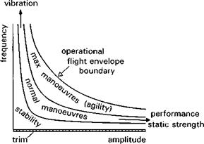
A convenient and intuitive framework for introducing this important topic is illustrated in Fig. 2.14, where the natural modelling dimensions of frequency and amplitude are used to characterize the range of problems within the OFE. The three fundamentals of flight dynamics – trim, stability and response – can be seen delineated, with the latter expressed in terms of the manoeuvre envelope from normal to maximum at the OFE boundary. The figure also serves as a guide to the scope of flight dynamics as covered in this book. At small amplitudes and high frequency, the problem domain merges with that of the loads and vibration engineer. The separating frequency is not distinct. The flight dynamicist is principally interested in the loads that can displace the aircraft’s

flight path, and over which the human or automatic pilot has some direct control. On the rotor, these reduce to the zeroth and first harmonic motions and loads – all higher harmonics transmit zero mean vibrations to the fuselage; so the distinction would appear deceptively simple. The first harmonic loads will be transmitted through the various load paths to the fuselage at a frequency depending on the number of blades. Perhaps the only general statement that can be made regarding the extent of the flight dynamicists’ domain is that they must be cognisant of all loads and motions that are of primary (generally speaking, controlled) and secondary (generally speaking, uncon­trolled) interest in the achievement of good flying qualities. So, for example, the forced response of the first elastic torsion mode of the rotor blades (natural frequency 0(20 Hz)) at one-per-rev could be critical to modelling the rotor cyclic pitch requirements correctly (Ref. 2.8); including a model of the lead/lag blade dynamics could be critical to establishing the limits on rate stabilization gain in an automatic flight control sys­tem (Ref. 2.9); modelling the fuselage bending frequencies and mode shapes could be critical to the flight control system sensor design and layout (Ref. 2.10).

At the other extreme, the discipline merges with that of the performance and structural engineers, although both will be generally concerned with behaviour across the OFE boundary. Power requirements and trim efficiency (range and payload issues) are part of the flight dynamicist’s remit. The aircraft’s static and dynamic (fatigue) structural strength presents constraints on what can be achieved from the point of view of flight path control. These need to be well understood by the flight dynamicist.

In summary, vibration, structural loads and steady-state performance traditionally define the edges of the OFE within the framework of Fig. 2.14. Good flying qualities then ensure that the OFE can be used safely, in particular that there will always be sufficient control margin to enable recovery in emergency situations. But control margin can be interpreted in a dynamic context, including concepts such as pilot-induced oscillations and agility. Just as with high-performance fixed-wing aircraft, the dynamic OFE can be limited, and hence defined, by flying qualities for rotorcraft. In practice, a balanced design will embrace these in harmony with the central flight dynamics issues, drawing on concurrent engineering techniques (Ref. 2.11) to quantify the trade-offs and to identify any critical conflicts.

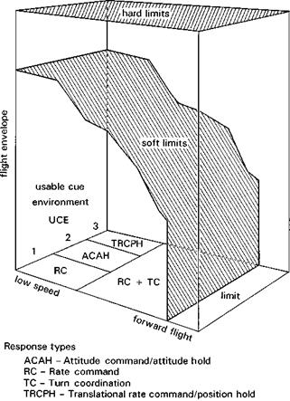
Figure 2.13 illustrates in composite form the interactional nature of the flight dynam­ics process as reflected by the four reference points. The figure, drawing from the parlance of ADS-33, tells us that to achieve Level 1 handling qualities in a UCE of 1, a rate response type is adequate; to achieve the same in UCEs of 2 and 3 require AC (attitude command) or TRC (translational rate command) response types respec­tively. This classification represents a fundamental development in helicopter handling qualities that lifts the veil off a very complex and confused matter. The figure also shows that if the UCE can be upgraded from a 3 to a 2, then reduced augmentation will be required. A major trade-off between the quality of the visual cues and the quality of the control augmentation emerges. This will be a focus of attention in later chapters. Figure 2.13 also reflects the requirement that the optimum vehicle dynamic characteristics may need to change for different MTEs and at the edges of the OFE; terminology borrowed from fixed-wing parlance serves to describe these features – task-tailored or mission-oriented flying qualities and carefree handling. Above all else, the quality requirements for flying are driven by the performance and piloting workload

demands in the MTEs, which are themselves regularly changing user-defined require­ments. The whole subject is thus evolving from the four reference points – the mission, the environment, the vehicle and the pilot; they support the flight dynamics discipline and provide an application framework for understanding and interpreting the mod­elling and criteria of task-oriented flying qualities. Continuing on the Tour, we address the first of three key technical areas with stronger analytical content – theoretical modelling.

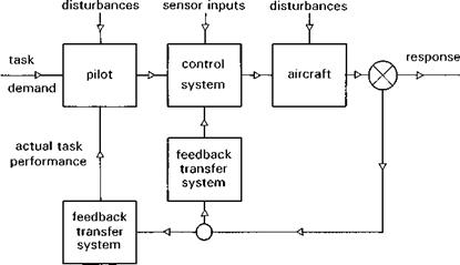
This aspect of the subject draws its conceptual and application boundaries from the engineering and psychological facets of the human factors discipline. We are con­cerned in this book with the piloting task and hence with only that function in the crew station; the crew have other, perhaps more important, mission-related duties, but the degree of spare capacity which the pilot has to share these will depend critically on his flying workload. The flying task can be visualized as a closed-loop feedback

system with the pilot as the key sensor and motivator (Fig. 2.12). The elements of Fig. 2.12 form this fourth reference point. The pilot will be well trained and highly adaptive (this is particularly true of helicopter pilots), and ultimately his or her skills and experience will determine how well a mission is performed. Pilots gather infor­mation visually from the outside world and instrument displays, from motion cues and tactile sensory organs. They continuously make judgements of the quality of their flight path management and apply any required corrections through their controllers. The pilot’s acceptance of any new function or new method of achieving an existing function that assists the piloting task is so important that it is vital that prototypes are evaluated with test pilots prior to delivery into service. This fairly obvious statement is emphasized at this point because of its profound impact on the flying qualities ‘pro­cess’, e. g., the development of new handling criteria, new helmet-mounted display formats or multi-axis sidesticks. Pilot-subjective opinion of quality, its measurement, interpretation and correlation with objective measures, underpins all substantiated data and hence needs to be central to all new developments. Here lies a small catch; most pilots learn to live with and love their aircraft and to compensate for deficiencies. They will almost certainly have invested some of their ego in their high level of skill and ability to perform well in difficult situations. Any developments that call for changes in the way they fly can be met by resistance. To a large extent, this reflects a natural caution and needs to be heeded; test pilots are trained to be critical and to challenge the engineer’s assumptions because ultimately they will have to work with the new developments.

Later in this book, in Chapter 6 and, more particularly, Chapter 7, the key role that test pilots have played in the development of flying qualities and flight control technology over the last 10 years will be addressed. In Chapter 8 the treatment of the topic of degraded handling qualities will expose some of the dangerous conditions pilots can experience. Lessons learnt through the author’s personal experience of working with test pilots will be covered.

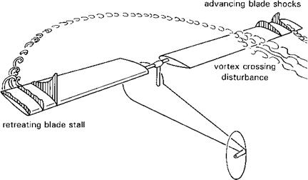
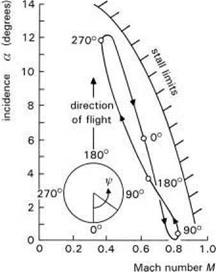
While aeroplanes stall boundaries in level flight occur at low speed, helicopter stall boundaries occur typically at the high-speed end of the OFE. Figure 2.9 shows the aerodynamic mechanisms at work at the boundary. As the helicopter flies faster, forward cyclic is increased to counteract the lateral lift asymmetry due to cyclical dynamic pressure variations. This increases retreating blade incidences and reduces advancing blade incidences (a); at the same time forward flight brings cyclical Mach number (M) variations and the a versus M locus takes the shape sketched in Fig. 2.10. The stall boundary is also drawn, showing how both advancing and retreating blades are close to the limit at high speed. The low-speed, trailing edge-type, high incidence (0(15°)) stall on the retreating blade is usually triggered first, often by the sharp local incidence perturbations induced by the trailing tip vortex from previous blades. Shock- induced boundary layer separation will stall the advancing blade at very low incidence (0(1-2°)). Both retreating and advancing blade stall are initially local, transient effects and self-limiting on account of the decreasing incidence and increasing velocities in the fourth quadrant of the disc and the decreasing Mach number in the second quadrant. The overall effect on rotor lift will not be nearly as dramatic as when an aeroplane stalls at low speed. However, the rotor blade lift stall is usually accompanied by a large change in blade chordwise pitching moment, which in turn induces a strong, potentially more sustained, torsional oscillation and fluctuating stall, increasing vibration levels and inducing strong aircraft pitch and roll motions.

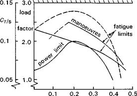
Rotor stall and the attendant increase in loads therefore determine the limits to forward speed for helicopters. This and other effects can be illustrated on a plot of rotor lift (or thrust T) limits against forward speed V. It is more general to normalize these quantities as thrust coefficient Ct and advance ratio д, where

^ T V

Ct = p(OR)2nR2 ’ Д = OR

where O is the rotorspeed, R the rotor radius and p the air density. Figure 2.11 shows how the thrust limits vary with advance ratio and includes the sustained or power limit boundary, the retreating and advancing blade lines, the maximum thrust line and the structural boundary. The parameter s is the solidity defined as the ratio of blade area to disc area. The retreating and advancing blade thrust lines in the figure correspond to both level and manoeuvring flight. At a given speed, the thrust coefficient can be increased in level flight, by increasing weight or height flown or by increasing the load factor in a manoeuvre. The manoeuvre can be sustained or transient and the limits will be different for the two cases, the loading peak moving inboard and ahead of the retreating side of the disc in the transient case. The retreating/advancing blade limits define the onset of increased vibration caused by local stall, and flight beyond these limits is accompanied by a marked increase in the fatigue life usage. These are soft limits, in that they are contained within the OFE and the pilot can fly through them. However, the usage spectrum for the aircraft will, in turn, define the amount of time the aircraft is likely (designed) to spend at different Ct or load factors, which, in turn, will define the service life of stressed components. The maximum thrust line defines the potential limit of the rotor, before local stall spreads so wide that the total lift reduces. The other imposed limits are defined by the capability of the powerplant and structural strength of critical components in the rotor and fuselage. The latter is an

advance ratio

————— advancing blade limit (drag rise)

————— retreating blade limit (blade stall)

Fig. 2.11 Rotor thrust limits as a function of advance ratio

SFE design limit, set well outside the OFE. However, rotors at high speed, just like the wings on fixed-wing aeroplanes, are sometimes aerodynamically capable of exceeding this.

Having dwelt on aspects of rotor physics and the importance of rotor thrust limits, it needs to be emphasized that the pilot does not normally know what the rotor thrust is; he or she can infer it from a load factor or ‘g’ meter, and from a knowledge of take-off weight and fuel burn, but the rotor limits of more immediate and critical interest to the pilot will be torque (more correctly a coupled rotor/transmission limit) and rotorspeed. Rotorspeed is automatically governed on turbine-powered helicopters, and controlled to remain within a fairly narrow range, dropping only about 5% between autorotation and full power climb, for example. Overtorquing and overspeeding are potential hazards for the rotor at the two extremes and are particularly dangerous when the pilot tries to demand full performance in emergency situations, e. g., evasive hard turn or pop-up to avoid an obstacle.

Rotor limits, whether thrust, torque or rotorspeed in nature, play a major role in the flight dynamics of helicopters, in the changing aeroelastic behaviour through to the handling qualities experienced by the pilot. Understanding the mechanisms at work near the flight envelope boundary is important in the provision of carefree handling, a subject we shall return to in Chapter 7.

It is convenient for descriptive purposes to consider the flight of the helicopter in two distinct regimes – hover/low speed (up to about 45 knots), including vertical manoeuvring, and mid/high speed flight (up to Vne – never-exceed velocity). The low – speed regime is very much unique to the helicopter as an operationally useful regime; no other flight vehicles are so flexible and efficient at manoeuvring slowly, close to the ground and obstacles, with the pilot able to manoeuvre the aircraft almost with disregard for flight direction. The pilot has direct control of thrust with collective and the response is fairly immediate (time constant to maximum acceleration 0(0.1 s)); the vertical rate time constant is much greater, 0(3 s), giving the pilot the impression of an acceleration command response type (see Section 2.3). Typical hover thrust margins at operational weights are between 5 and 10% providing an initial horizontal acceleration capability of about 0.3-0.5 g. This margin increases through the low-speed regime as the (induced rotor) power required reduces (see Chapter 3). Pitch and roll manoeuvring are accomplished through tilting the rotor disc and hence rotating the

fuselage and rotor thrust (time constant for rate response types 0(0.5 s)), yaw through tail rotor collective (yaw rate time constant 0(2 s)) and vertical through collective, as described above. Flight in the low-speed regime can be gentle and docile or aggressive and agile, depending on aircraft performance and the urgency with which the pilot ‘attacks’ a particular manoeuvre. The pilot cannot adopt a carefree handling approach, however. Apart from the need to monitor and respect flight envelope limits, a pilot has to be wary of a number of behavioural quirks of the conventional helicopter in its privileged low-speed regime. Many of these are not fully understood and similar physical mechanisms appear to lead to quite different handling behaviour depending on the aircraft configuration. A descriptive parlance has built up over the years, some of which has developed in an almost mythical fashion as pilots relate anecdotes of their experiences ‘close to the edge’. These include ground horseshoe effect, pitch-up, vortex ring and power settling, fishtailing and inflow roll. Later, in Chapter 3, some of these effects will be explained through modelling, but it is worth noting that such phenomena are difficult to model accurately, often being the result of strongly interacting, nonlinear and time-dependent forces. A brief glimpse of just two will suffice for the moment.

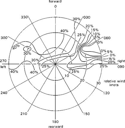
Figure 2.7 illustrates the tail rotor control requirements for early Marks (Mks 1-5) of Lynx at high all-up-weight, in the low-speed regime corresponding to winds from

different ‘forward’ azimuths (for pedal positions <40%). The asymmetry is striking, and the ‘hole’ in the envelope with winds from ‘green 060-075’ (green winds from starboard in directions between 60° and 75° from aircraft nose) is clearly shown. This has been attributed to main rotor wake/tail rotor interactions, which lead to a loss of tail rotor effectiveness when the main rotor wake becomes entrained in the tail rotor. The loss of control and high power requirements threatening at this particular edge of the envelope provide for very little margin between the OFE and SFE.

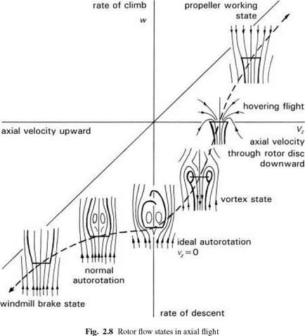
A second example is the so-called vortex-ring condition, which occurs in near­vertical descent conditions at moderate rates of descent (0(500-800 ft/min)) on the main rotor and corresponding conditions in sideways motion on the tail rotor. Figure 2.8, derived from Drees (Ref. 2.7), illustrates the flow patterns through a rotor operating in vertical flight. At the two extremes of helicopter (propeller) and windmill states, the flow is relatively uniform. Before the ideal autorotation condition is reached, where the induced downwash is equal and opposite to the upflow, a state of irregular and strong vorticity develops, where the upflow/downwash becomes entrained together in a doughnut-shaped vortex. The downwash increases as the vortex grows in strength,

leading to large reductions in rotor blade incidences spanwise. Entering the vortex-ring state, the helicopter will increase its rate of descent very rapidly as the lift is lost; any further application of collective by the pilot will tend to reduce the rotor efficiency even further – rates of descent of more than 3000 ft/min can build up very rapidly. The consequences of entering a vortex ring when close to the ground are extremely hazardous.