Our heavyweight helicopter equal in the world does not have
In Rostov started production of the most load-lifting rotary-wing car The Russian holding «Helicopt[...]

Everything about aircrafts and helicopters. News and events in aviation worldwide. Civil, transportation, military helicopters and airplanes.

Everything about aircrafts and helicopters. News and events in aviation worldwide. Civil, transportation, military helicopters and airplanes.

Everything about aircrafts and helicopters. News and events in aviation worldwide. Civil, transportation, military helicopters and airplanes.

Everything about aircrafts and helicopters. News and events in aviation worldwide. Civil, transportation, military helicopters and airplanes.


Important new research on model aerofoil section design was carried out at Princeton University between 1986 and 89 by Michael Selig, John Donovan and David Fraser.
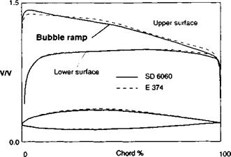
Using the aerofoil design program developed by Eppler and Somers, combined with that of Drela and Giles, which in some respects has been found more accurate for predictive purposes at low Reynolds numbers, a family of entirely new profiles was designed and tested in the Princeton wind tunnel. The theoretical basis of the new series, all carrying the prefix SD followed by a four digit number (e. g., Selig-Donovan SD 7032) is adjustment of the pressure distribution over the upper surface of the profile by introduction of a ‘bubble ramp’. (The SD profiles should be distinguished from the earlier series ‘S’ designed by Selig, mentioned in Section 9.8 above.)
If the transition from falling pressure to rising pressure over the upper surface of the wing is too sudden and the pressure recovery gradient aft too steep, a separation bubble is almost sure to form. If, however, the rising pressure gradient can be smoothed out and made very gradual, transition in the boundary layer from laminar to turbulent flow may be achieved without separation.
The SD profiles for models have the recovery aft of the lowest pressure point carefully
|
Fig. 9.18 Velocity/pressure distributions, SD 6060 compared with Eppler 374 at a lift coefficient of 0.55
|
|
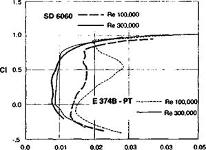
Fig. 9.19 Comparison drag curves for the Eppler 374 and SD 6060 tested at Princeton at two Reynolds numbers
|
Cd
calculated to be as smooth and even as possible with no changes in the rate of change until very close to the trailing edge. The long, gentle pressure recovery zone is termed the bubble ramp. It should be compared with the very abrupt change in the upper surface pressure distribution shown for the NACA 6 Series profiles (Fig. 9.3 above). A comparison of the SD 6060 profile with the well known Eppler 374 is shown in Fig. 9.18. The wind tunnel results show a very worthwhile drag reduction, especially noticeable at the lower Re (Fig. 9.19).
Further brief discussion of the Princeton wind tunnel test work appears in the next chapter.
Of particular importance has been the publication of Professor Richard Eppler’s computer programme, in co-operation with Dan Somers. This programme was developed in order to enable a wing profile to be designed exactly to fit any required specification and it has been used with excellent results for full-sized as well as model aeroplane and sailplane aerofoils. It has also been applied to model wing sections, notably by Rolf Girsberger in Switzerland, Helmut Quabeck and Martin Hepperle in Germany, and Michael Selig in the U. S.A. (Note, the HQ profiles designed for models by Quabeck
Seporation bubble worning
д upper surface
![Подпись: Theory Re - 10s E 6V 8Л5І Fig. 9.16 Drag polar of Eppler 64, 8.5% thick aerofoil, as measured in wind tunnel, compared with theoretical prediction at Reynolds number 100 000. Note where theory predicts separation bubbles on both upper and lower surfaces, measured drag is far greater. Note also that the Cd scale does not start at zero. (Chart published first by R. Eppler in his paper read at the R.Ae.Soc. Conference, October 1986].](/img/3131/image150_4.gif) |
t U t 8A5X v l°wer surface
Fig. 9.17 Theory and test of the Eppler 65, 8.86% thick profile, at Re 100 000 and 200 000.
Note the different scales of drag, starting at 0.01 and 0.0 respectively.
 |
Separation bubble warning л upper surface v lower surface
|
E 65 8.86* |
 |
Separation bubble warning д upper surface v lower surface
should not be confused with the Horstmann and Quast HQ series for full-sized aircraft.)
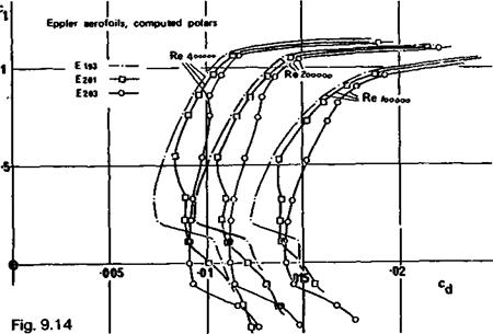
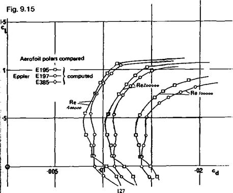
The Eppler programme, when applied to very low Re numbers, gives warning when laminar separation bubbles on the wing are likely to cause significant departures of the actual lift and drag figures achieved in flight, from the theoretical predictions. Drag polar curves similar to those of Figures 9.14 and 9. IS now usually appear with ‘bubble warning’ tags at various points. Practical wind tunnel tests, mostly by Dieter Althaus at Stuttgart, demonstrate that wherever a bubble warning appears on the computed charts, the drag curve will depart quite seriously from the computed figures, almost invariably moving to the high drag side.
Some of the results are illustrated in Figures 9.16—9.18. These have been published by Eppler himself. In Figure 9.16, a drag polar for the Eppler 64 profile is shown for Reynolds number 100,000. The computer predicts bubble separation over most of the operating range of the aerofoil. The two curves diverge markedly, especially where the computer programme predicted the minimum drag coefficient. Near this location on the curve, separation bubble warnings appear on both upper and lower surfaces of the wing (indicated by overlapping triangles making a six pointed star). Agreement of the theoretical curve with the measured one is better at higher Re.
In Figure 9.17 results are shown for the Eppler 65 at two different Re numbers. At the higher Re of200,000, agreement of theory and measurement is not too bad although far from perfect. The computer predicts separation bubbles over most of the usable range of C| values. At the lower Re of 100,000, the two curves match nowhere except over a very narrow range at high cj, very close to the stall. Again this is no surprise in view of the bubble warnings.
Eppler concludes that while the bubble warnings on the computed polars are useful, their true significance is that modellers cannot rely on the computed drag curves of any aerofoil produced by these methods when the warning tags appear. These remarks apply equally to profiles designed by others using the Eppler programme or equivalents to it. Profiles by Helmut Quabeck, Rolf Girsberger and Michael Selig have been well proved in practice, as have those of Eppler himself, but at low Re they do not perform as efficiently as expected. Laminar separation bubbles do occur on all of them and do affect the drag. (Eppler points out that E65 is of theoretical interest only and is not recommended for practical use.)
It must be emphasised that at Re below 500,000 boundary layer flows and separation bubbles are very complicated and up to the time of writing, mathematical and theoretical analysis has not been able to deal adequately with them.
Since the first edition of this book was published in 1978, a great deal of research of both theoretical and practical kind has been done. Leading roles in this have been taken
|
|
|
|
by universities at Stuttgart and Brunswick (Germany), Delft (Netherlands), Southampton and Cranfield (U. K.) and Notre Dame (U. S.A.), with other important contributions by
S. J. Miley and R. H. Liebeck, and D. Somers and S. M. Mangalam at NASA, where Walter Pfenninger also has worked for many years. Many of the most significant results were presented in the form of papers and summaries in academic journals, and at conferences, especially one at Notre Dame in 198S and a larger international meeting at the Royal Aeronauticid Society in London in October 1986. Although often of a highly technical and mathematical kind, many of these reports contain information of great significance for model fliers and should be consulted for detailed information on specific points. (See the list of references following Chapter 10). Some of the work remains unpublished or is available only from technical libraries or direct from the university departments concerned.
All these features of the NACA ‘6’ profiles were recognised in the 1950s by designers of full-sized sailplanes. The great width of the low drag range of the thicker profiles at sailplane Re led to the adoption of profiles such as the NACA 633618 and 633621 for such successful types as the Ka 6 and Skylark series respectively. The performance, particularly at high speeds, was a vast improvement on earlier types such as the Olympia and Weihe which had thinner wings (Gdttingen 549) but with turbulent flow. However, although the new profiles were cambered for ci 0.6, and worked efficiently up to ci 0.9 and
|
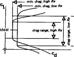
Fig. 9.7 The low drag range at high and low Re |
a little beyond (because of the wider low drag bucket at low Re), there were still problems at higher c|. Cambering the wings more led to flow separation at the low speed end of the range, and tended to spoil the high speed performance below сі 0.3. How the ‘6’ series profiles perform at Re lower than 700,000 is hardly known, since few wind tunnel tests have been carried out below this figure. They have been successfully used on man – powered aircraft and a few of the better hang gliders. They should perform very well on fast models, providing the correct camber value is chosen. The temptation to thin the profile on a speed model too much should be resisted. For practical racing, a thicker profile is less sensitive to errors and enables turns to be flown economically without danger of sudden increases of drag.
For scale model sailplanes, the great thickness of the typical ‘6’ series aerofoils used on the prototypes may cause difficulties. Such aerofoils still have a critical Re below which flow will separate and not re-attach. Unless the model is very large in chord, the profile, while it should retain a laminar flow thickness form, will require thinning down. Of course, full-size sailplanes have very narrow, high aspect ratio wings. The very thick aerofoils on such types as the Skylark 2,3 and 4 are not suitable for small models of these aircraft Their wide low drag range cannot, therefore, be employed on small models. The same applies to more recent sailplane designs which still may have aerofoils of 17% thickness, with even higher a. r. Earlier, pre-laminar flow sailplanes make more suitable prototypes for scale modelling since they usually had lower aspect ratios (broader chord), and thinner aerofoils. However, some of these aerofoils had unduly large leading edge radii and hence high critical Re. Scale model sailplanes should, in general, be as large as possible if the same aerofoil is to be used on the prototype. Otherwise the flying performance will be very disappointing. The same argument applies, of course, to all scale models, but with full-sized powered aircraft speed range is less important so the aerofoils used are usually as thin as possible for the sake of efficiency at one speed. Hence the scale aerofoil tends to have a lower critical Re and there is more prospect of success for the small model. Also, with most prototypes, there are irregularities in the neighbourhood of the leading edge which allow the modeller to ‘turbulate’ the airflow. This applies with special force to so-called ‘peanut’ scale models. Some of the best full-sized prototypes for such models are the very early aeroplanes which had thin wings resembling the curved plate profiles of the previous chapter.
|
|
In designing aerofoils the next important steps forward were taken by R. Eppler and F. X. Wortmann, working independently in Germany during the 1950s and 60s. Eppler’s early full-sized sailplane profiles should not be confused with those he has more recently produced for models. They are designed on different principles, and may be distinguished by their more complex-seeming designations, such as EA 8 (-1) 1206. (One such experimental section was, unlike the others, intended for models, and has been tested by Kraemer in the wind tunnel. The results are given in Appendix 2, the Gottingen number being 804.) On full-sized sailplanes, the earlier Eppler profiles are now rarely employed, although in their day they were a distinct improvement, as far as speed range was concerned, over the NACA ‘6’ profiles. Eppler argued that sailplanes never operated at one design value or ideal Cl, but were always either climbing in thermals at minimum sink corresponding to high cj, or ‘penetrating’ at low Cl (see Fig. 4.3). Rather than trying to widen the low drag range of NACA profiles, he designed profiles which in effect split the bucket into two, as indicated in Figure 9.8. The first glassfibre sailplane, the record breaking Phonix, had a profile of this type, and so did the subsequent Phoebus series. The original (wooden) Standard Austria design with the NACA 652415 profile was much improved when it was re-winged with an Eppler profile to create the SH 1, even though this profile was slightly thicker. Eppler achieved his results by designing for laminar flow on one surface of the wing at high angle of attack, and the other surface at low angles of attack. In between, both surfaces were turbulent, but he argued that this hardly mattered. Flight measurements on the Phonix confirmed his theoretical expectations. It is, however, doubtful if these profiles are of value in modelling, and they will not be discussed further here.
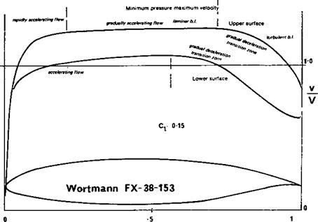
F. X. Wortmann’s work followed a different line.* On full-sized sailplanes, at the 1974 World Championships every sailplane competing had Wortmann aerofoils. The thinner examples work well on larger model sailplanes. Some of the less cambered Wortmann profiles might also be superior to the NACA ‘6’ series for racing powered models. Wind tunnel results are promising. For gliders Wortmann concentrated on widening the low drag bucket of laminar flow profiles, using electronic computer techniques to achieve the desired grading of the velocity distribution curves.
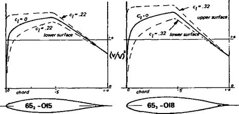
The velocity distributions of the NACA profiles, as shown in Figure 9.3, exhibit a sharp kink in the curve at the maximum velocity/minimum pressure point A straight line was drawn from here and the profile thickness designed to produce this sharp change. The airstream velocity after the sudden onset of deceleration slows down at a steady rate all the way. At low Re the separation bubble forms, on such a profile, almost immediately behind the minimum pressure point. After re-attachment, the turbulent boundary layer steadily loses momentum, and although it does not separate immediately, as it becomes slower and slower it loses its ability to maintain contact with the wing, and some separation is very likely before the trailing edge is reached. This separation marks the limit of the low drag bucket At lower Re, to take advantage of the natural tendency to greater laminar flow, the sharp kink in the curve, Wortmann argued, should be smoothed out. The laminar boundary layer would then be able to persist further behind the minimum pressure point, and if the flow deceleration over this portion of the wing was gradual, it might be capable of continuing even as far as 70% of the way to the trailing edge. Transition, with separation bubble, would eventually come, however, and here again a different principle was needed. After transition, the boundary layer has plenty of momentum (providing it has not completely separated), and can remain attached to the wing even against a sharp pressure gradient As it nears the trailing edge, the energy * Professor Wortmann died in 1985.
available is less, so it should be required to fight a less severe gradient. The result of this reasoning in terms of graded velocity profile for a man-powered aircraft aerofoil is shown in Figure 9.9 and for a high speed aerofoil in Fig. 9.10.
Profiles designed around these principles have been extensively tested in wind tunnels and in flight, and the expected results are achieved. The low drag bucket is no longer so flat-bottomed, i. e. there is some increase of cd as the ci rises above the designed value, but * the total width of the ‘bucket’ is considerably more than that of equivalent NACA profiles. Performance at high ci is better. Ordinates for the thinner types of Wortmann profile are given in Appendix 3. The thicker profiles are probably not good for models. The FX 63-13.7 has been tested extensively by a number of different research organisations over a considerable range of Re numbers. It is too strongly cambered for most model applications, since it was designed for a man-powered aircraft. A number of flapped sections is also given. The flapped profiles give good results only if the flap is of the correct size, as specified, and the flap should be set correctly for each flying speed. If this is not done, the profile is actually less efficient than the un-flapped versions. However, with flaps correctly used and gaps sealed, the width of the low drag range is even further increased.
The Wortmann aerofoils are mutually compatible with one another for use in tapered wings. In particular the FX 60-126 was intended for use at wing tips. It has a late stall and so may be employed without washout, or only a very small amount Large model sailplanes have been successful with these profiles. The FX 60-100, a thinner version, has been very popular with model fliers. At Re lower than 100 to 200 thousand the behaviour of most Wortmann sections remains to be investigated.
|
Fig. 9.10 Calculated velocity gradients over a Wortmann high speed aerofoil. 15.9% thick |
The aerofoils designed specifically for models by R. Eppler have achieved great popularity. They range from thin, highly cambered profiles intended for free-flight ; duration models, to much thicker sections for large sailplanes. By an extension of his < earlier thinking, Eppler designed these profiles so that a pressure gradient favourable for laminar flow is preserved as far as possible on at least one surface of the wing – the upper ■ surface at low angles of attack, die lower surface at high angles. However, at some intermediate angle, instead of both surfaces being turbulent (as with his full-sized profiles, Fig. 9.7), there is a range of angles over which laminar flow should exist on both surfaces for some distance. Examples, in terms of computed velocity distributions, are shown in Figures 9.11 – 9.13. At 9 degrees angle of attack the E 203 profile has an accelerating boundary layer on the underside up to about 35% of the chord. (The speed of flow remains less than that of the mainstream, to produce positive pressure.) After the maximum velocity point, the decrease is very gradual, so there is every chance for the laminar boundary layer to persist for some distance, and then become turbulent On the
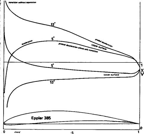
r This profile is designed for large models, and there should be no danger of premature stall. ‘ After the separation bubble the boundary layer re-attaches, overcomes the adverse I pressure gradient and remains attached – At zero angle of attack, close to the zero lift angle I for this profile, the upper surface has laminar flow while the underside now has the early I pressure peak and gradual deceleration thereafter. At angles between these two, the jj profile should have extensive laminar flow on both surfaces, and the minimum profile drag N will be achieved. This is a relatively high speed profile. A similar set of curves for a lower і speed profile, the E 385, is shown in Figure 9.12.
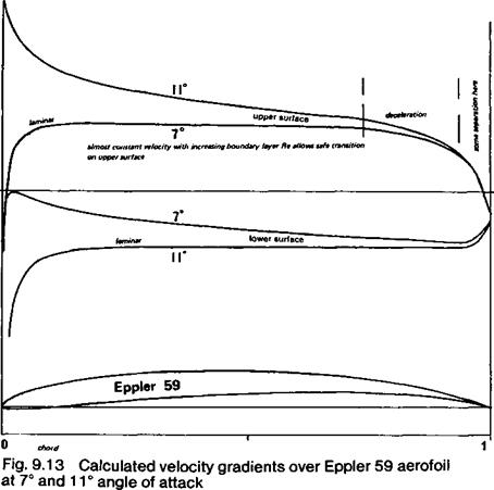
г For very low Re, the thin profiles E 58 and 59 have been designed. The likelihood of I flow separation at low Re is much greater, as stressed in Chapter 7, and Eppler admits I that some separation does occur even on these very thin profiles due to the very sharp [‘ decrease of flow speeds near the trailing edge on the upper surfaces (see Fig. 9.13).
? However, at the designed angle of attack, the computed velocity and pressure gradient on » the upper side is almost constant over a large proportion of the chord. This allows the jf laminar boundary layer to continue as far as possible and make a safe transition to
|
Fig. 9.12 Calculated velocity gradients over Eppler 385 aerofoil at 5° and 13° angle of attack |
|
|
turbulent flow either as or before the deceleration begins. Although, as with all thin, highly cambered profiles, such wings will be critical in trimming and will require large stabilisers, the performance gain should be worthwhile. This is, of course, still subject to the limitation that profile drag on a model at low speed is relatively much less significant than aspect ratio. Unlike the ‘turbulent flow’ aerofoils of the previous chapter, these profiles should be built without leading edge waviness. Sheet balsa covering or even solid balsa construction at least over the front half of the wing should be regarded as essential. Theoretical drag polars of several Eppler aerofoils are given in Figure 9.14 and 9.15.
 |
In Figure 9.5 is shown a typical curve of profile drag plotted against ci for any of the NACA 6 series aerofoils. At the design ci, drag is much lower than for an orthodox or old – fashioned section. On either side of this value there is a low drag range or ‘bucket’ in the graph, so that small departures from the ideal operating conditions cause no change in profile drag coefficient At either side of the low drag bucket, on one surface or another, the velocity distribution changes and the boundary layer becomes turbulent, with an associated sharp rise in drag. In the NACA designations of these aerofoils, the third digit,
of thick and thin profiles
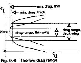 |
usually written as subscript thus: NACA 643418, indicates the width of the low drag bucket, in this case 0.3 ci on either side of the ideal designed value for the profile. A profile with the subscript 3 as above, designed for a ci of 0.4, will work efficiently at c) down to 0.1 and up to 0.7. (Note, however, that constant drag coefficient does not mean constant drag force – the higher speed associated with lower Cl of the wing increase drag force at a constant Cd – see Chapter 2.) The fourth digit of the aerofoil number gives the design ideal lift coefficient, in tenths, and the final two figures give the profile thickness as a percentage of the chord.
As already noted from the velocity profiles of the thick profiles of Figure 9.3, favourable flow conditions are preserved on thicker aerofoils over a greater range of ci than on thin ones. The absolute minimum drag of a thick profile is slightly more than for a thin section of similar camber, but the drag bucket of the thick profile is wider. This is indicated in Figure 9.3. Such a thick wing has a wider speed range, and, in the case, for example, of a racing model, will be less affected by slight inaccuracies of flying, and less slowed down in steep turns, than a model with thin wing and higher maximum speed straight and level.
As the Reynolds number is reduced, so long as flow remains super-critical (i. e. reattachment after the separation bubble), the natural tendency for laminar flow to persist shows up. The minimum drag of the laminar flow profile is slightly higher (because the relative viscosity of the air at low speeds is greater compared with the density-speed – chord factors), but the boundary layer, after passing the maximum velocity point on the wing, remains laminar for a greater distance and this has the effect of widening the drag bucket slightly. The result is shown diagrammatically in Figure 9.6.
Aerofoils are no longer designed by ‘cut and try’ methods, but are worked out to fit their special purposes. The first substantial gains achieved were the NACA ‘6’ series aerofoils developed before and during the Second World War. They were used, in slightly modified form, first on the P-З I ‘Mustang’ fighter. These aerofoils were designed to achieve very low profile drag by preserving laminar flow over as much of the wing as possible. The improvements in practice were less than hoped for, because of the inaccuracies of the wings in service, but there were genuine overall benefits. The main method of achieving
Fig. 9.2 cont.
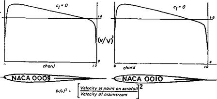
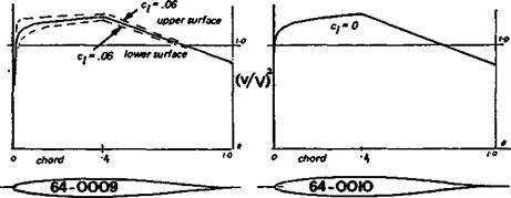
NACA 0009 LE RADIUS 0.89 PERCENT NACA 0010 LE RADIUS 1.10 PERCENT
|
CHORD |
UPPER |
CHORD |
LOWER |
CHORD |
UPPER |
CHORD |
LOWER |
|
STATION |
SURFACE |
STATION |
SURFACE |
STATION |
SURFACE |
STATION |
SURFACE |
|
XU |
YU |
XL |
YL |
XU |
YU |
XL |
YL |
|
0.000 |
0.000 |
0.000 |
0.000 |
0.000 |
0.000 |
0.000 |
0.000 |
|
.600 |
1.010 |
.600 |
-1.010 |
.600 |
1.120 |
.600 |
-1.120 |
|
.800 |
1.170 |
.800 |
-1.170 |
.800 |
1.250 |
.800 |
-1.250 |
|
1.250 |
1.420 |
1.250 |
-1.420 |
1.250 |
1.578 |
1.250 |
-1.578 |
|
2.500 |
1.961 |
2.500 |
-1.961 |
2.500 |
2.178 |
2.500 |
-2.178 |
|
5.000 |
2.666 |
5.000 |
– 2.666 |
5.000 |
2.962 |
5.000 |
– 2.962 |
|
7.500 |
3.150 |
7.500 |
-3.150 |
7.500 |
3.500 |
7.500 |
– 3.500 |
|
10.000 |
3.512 |
10.000 |
-3.512 |
10.000 |
3.902 |
10.000 |
– 3.902 |
|
15.000 |
4.009 |
15.000 |
-4.009 |
15.000 |
4.455 |
15.000 |
-4.455 |
|
20.000 |
4.303 |
20.000 |
-4.303 |
20.000 |
4.782 |
20.000 |
-4.782 |
|
25.000 |
4.456 |
25.000 |
– 4.456 |
25.000 |
4.952 |
25.000 |
-4.952 |
|
30.000 |
4.501 |
30.000 |
-4.501 |
30.000 |
5.002 |
30.000 |
-5.002 |
|
40.000 |
4.352 |
40.000 |
– 4.352 |
40.000 |
4^37 |
40.000 |
-4.837 |
|
50.000 |
3.971 |
50.000 |
-3.971 |
50.000 |
4.412 |
50.000 |
-4.412 |
|
60.000 |
3.423 |
60.000 |
– 3.423 |
60.000 |
3.803 |
60.000 |
– 3.803 |
|
70.000 |
2.748 |
70.000 |
– 2.748 |
70.000 |
3.053 |
70.000 |
– 3.053 |
|
80.000 |
1.967 |
80.000 |
-1.967 |
80.000 |
2.187 |
80.000 |
-2.187 |
|
90.000 |
1.086 |
90.000 |
-1.086 |
90.000 |
1.207 |
90.000 |
-1.207 |
|
95.000 |
.605 |
95.000 |
– .605 |
95.000 |
.672 |
95.000 |
– .672 |
|
100.000 |
.095 |
100.000 |
– .095 |
100.000 |
.105 |
100.000 |
– .105 |
Note that the ordinates of the 9% thick profile are exactly 90% of the 10% profile. NACA four-digit symmetrical sections may alwaysbe scaled up or down to different thicknesses by simple arithmetic.
|
|
|
|
|
|
|
|
|
|
![]()
the lower drag was to employ aerofoil thickness forms similar to those shown in Figure 9.3. As the velocity diagrams show, at zero angle of attack the maximum velocity/: minimum pressure point on these profiles is at 40% or 50% of the chord. Other thickness I forms were designed with this point further back or further forward. The second digit of an, NACA profile designation, such as the 4 in 643618, indicates the position of the maximum velocity point The boundary layer, on a suitably smooth wing, will remain : laminar to a point somewhere aft of the 40% chord position on such an aerofoil. (By і suitably smooth is meant a wing free from ripples, humps or hollows rather than one which is highly polished.) As shown in Figure 9.3, at small angles of attack the velocity ‘ distribution on both surfaces is favourable for laminar flow back to the 40% point, the 9% thick profile at ci of.06. The thicker profile, 652015 shows that laminar flow is preserved on both sides up to a ci of 0.22. This is of great importance. A thicker wing at a high angle of attack may have greater percentage of laminar flow and hence lower drag than a thin profile. (Compare also the 653018 profile.) This applies equally to cambered profiles. If j one of the symmetrical sections of Figure 9.3 is cambered round the NACA a = 1 mean line, the basic character of the velocity distribution, and hence laminar flow, is not І changed. Figure 9.4 shows the results in graphical form. The amount of camber given to ‘ the profile is determined by the desired operational Cl, as described in Chapter 7. At this value, laminar flow prevails over both upper and lower surfaces, up to the peak velocity ■: position and slightly beyond it. At a higher angle of attack, the velocity graph resembles that of Figure 9.4(b). Transition on the upper surface occurs futher forward. There may even be flow separation further aft, but this is not important since the aircraft is not intended to operate far from its designed Cl – The result in terms of drag at the design ci of the profile is very substantial improvement
9.1 VELOCITY AND PRESSURE DISTRIBUTIONS
Aeromodelling has undergone a revolution since the time of F. W. Schmitz. Free flight models still operate close to critical Reynolds number conditions but radio controlled models, especially the larger sailplanes, high speed racers and aerobatic models are usually outside the danger area. Many such models fly quite successfully with profiles similar to the Clark Y or Gdttingen 796 and it is obvious that problems of sub-critical flow separation have been left behind. Part of the reason for this is that such models do not usually fly at very high angles of attack. As Schmitz’s results showed, a profile like the N-60 operated efficiently at a low angle of attack but stalled early even when operating, nominally, above its critical Re. The same thing was found on the Go 801, separation problems at high angles of attack did not entirely disappear until about Re 170,000. Modellers have put up with the premature stall of such profiles. Performance at higher speeds is quite good. The pylon racing model is in any case operating most of the time at Re’s quite comparable with those of full-sized sailplanes and even some light aeroplanes. Very great improvements in performance have been achieved in full-sized sailplanes, and some powered aircraft, by the use of so-called laminar flow profiles. The advantage in terms of saving skin friction are very large, especially at high speeds where profile drag becomes of major importance (Fig. 4.10). Early work in this area by the Low Speed Aerodynamics Research Association has been largely overlooked by modellers, but the aerofoils LDC2 and LDC3M produced were used on some models at the time, about 1948, when they first appeared.
As described in Chapter 3, on any wing, the boundary layer will be laminar at first near the leading edge, but will make a transition to turbulent flow when it reaches the critical boundary layer Re. The value of this critical Re will depend on the quality of the wing surface. Many full-sized aircraft have poor surfaces. Even if highly polished, there are waves and ripples in the skin caused by rivet tension and humps created by stiffeners and spars. It is very difficult to preserve laminar flow over such a wing for more than a few centimetres near the extreme leading edge, and even when great efforts are made to achieve an accurate profile, the large Reynolds number associated with the high flight speed and large wing chord, promotes early transition. The smallest defect in the surface, even a fly speck or the crushed body of an insect, can cause transition. For these and similar reasons designers of full-sized light aeroplanes have not been able to achieve all the benefits of low drag, laminar flow, and many still prefer to use relatively old-fashioned profiles. However, as the Reynolds number falls, the chances of preserving laminar flow over more of the wing increase. Small defects that, at higher velocities, cause transition,
may be over-ridden by the relatively more viscous boundary layer, and if wings can be made accurately, as they are in modem full-sized sailplanes, the aerodynamicists’ predictions, based on theoretical studies and wind tunnel tests, come true. The problem for modellers is the reverse of that for the turbulent flow aerofoils. At sub-critical Re, turbulators and protrusions caused by spars may improve performance by forcing transition in the boundary layer. Laminar flow models should seek to maintain profile accuracy at least as far back as the point where the boundary layer will make its transition naturally. The standard of precision required is, because of the low Re, less than that needed for the full-sized aircraft.
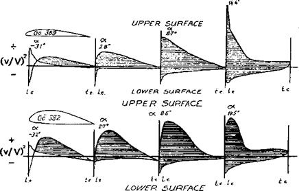
Providing the wing surface is smooth, a laminar boundary layer will tend to prevail as long as the speed of flow is rising under the influence of the low pressure area above the wing (Fig. 3.5). Behind the minimum pressure point the laminar flow persists for some distance but then a separation bubble forms and (providing super-critical Re prevails), the flow re-attaches as a turbulent boundary layer. In Figure 9.1 velocity measurements made on two wing profiles are shown. These show how the speed of flow over the upper and lower surfaces vary at different angles of attack. On the Gottingen 389, for example, at 2.8 degrees angle, the flow on the upper surface increases rapidly to a maximum within the first ten percent of the wing chord. Laminar flow will persist up to this point and a little way beyond it, but then transition will occur and turbulent, high drag flow covers most of the wing. At a lower angle of attack, -3.1 degrees, the maximum velocity point on the upper side is somewhat further back, but at higher angles it moves forward so that near the stall, at 14.6 degrees, the whole upper surface is in turbulent flow. Meanwhile, on the underside the velocity peak of the upper surface is opposed by a velocity decrease close to the leading edge, and thereafter the air accelerates towards the trailing edge. Transition
|
Fig. 9.1 Velocity profiles of two G6ttingen aerofoils OC
|
|
|
will already have taken place and the boundary layer will be turbulent. At the more negative angles of attack, the roles of upper and lower surfaces are reversed as the wing begins to ‘lift’ downwards.
The Gottingen 382 profile is a thicker version of the 389, but the velocity measurements show important differences. At 2.7 degrees angle, the velocity maximum on the upper side is about ten percent further aft than on the thinner profile, and even near the stall there is a likelihood for laminar flow back to about ten percent before the velocity decrease causes transition.
The details of the velocity of airflow over a wing depend on both its thickness form and its camber. The typical, pre-1940 aerofoils of Figure 9.1 and others of the same vintage, such as the Clark Y, N-60, etc. were designed around what was then thought to be the ideal form for any streamlined body. The same basic shape, thickened or thinned appropriately, was used for strut fairings, streamlined wires, tailplane and fin profiles, wheel spats and whole airship hulls. Typical ordinates are given in Figure 9.2 which refer to the NACA ‘four digit’ aerofoils. The velocity distribution graphs given with the profiles show that at zero angle of attack, the velocity peak (and hence minimum pressure point) on both surfaces is reached at about ten percent of the chord. A short distance aft of this, transition to turbulent flow occurs. Cambering changes this basic feature only slightly; such profiles are fundamentally incapable of preserving laminar airflow over much of the wing.
In measurements of boundary layers in low turbulence wind tunnels, it has been recognised for some time that noise alone can cause a delicate boundary layer flow to change sharply. Noise generated by the fan or motor of a wind tunnel can provoke early transition of a laminar boundaiy layer, and even the sound of someone walking past the test section may cause a change. Elaborate tests have been made with artificially generated sounds of varying pitch and volume, which show that separation and stalling can to some degree be controlled by this means. Sound is, basically, a series of small compression waves in the air and this may be enough to change the microscopic turbulence. Alternatively, the air noise may cause sympathetic vibrations in the solid wing skin, which could cause the boundary layer flow to change.
In practical model flying it is quite likely that the noise and vibrations caused by the engine and propeller cause the boundary layer to make transition to turbulence sooner than would occur on a sailplane, for instance. (It is highly unlikely that shouting, screaming or even singing at a model sailplane will have any effect!)
9
The fineness of the tape used for turbulators in all wind tunnel testing is worthy of note. Modellers have sometimes employed much thicker ones, sometimes using strips of limn or 1.5mm balsa where thicknesses one tenth of this should be sufficient Turbulators, or; invigorators, which are too thick can cause flow separation rather than improving the boundary layer conditions.
■І
8.3 ZIG ZAG TURBULATORS
There is much to be said for laying the tuibulator tape in zig-zag fashion. Tests at Delft і University have shown that a zig zag tape tuibulator just ahead of the separation point on the wing has a better effect than a straight strip. Hie best spacing of the zig zags is a matter i for experiment on a given wing. The best results are obtained when there is a definite { relationship between the natural tendency of the flow within the separation bubble to develop waves and small, chordwise vortices (see paragraph 3.9). The modeller is unlikely to know what this is without very costly tunnel tests and some calculation, so trial and error is the likely way of discovering the optimum arrangement Possibly pinking shears of different sizes could be used to produce tapes for trial.
8.4 PNEUMATIC TURBULATORS 1
Perforations, such as a row of pin holes through the wing skin instead of a tape strip, can | act as a tuibulator. 3
The air pressure inside a wing is usually somewhat greater than that on the upper 1 surface, so air is drawn through the perforations and injected into the boundaiy layer. Ibis ] in effect trips the flow and may be sufficient to make it tuibulent (The effect was first j noticed by M. M. Gates in wind tunnel tests carried out in the 1950s.) Many full-sized і sailplanes also use pneumatic boundary layer control, especially on the underside of the wing near the trailing edge, where a separation bubble commonly forms. High pressure air is taken in by a small intake, positioned under the wing, and this raises the pressure in the і hollow chamber inside the wing. Very fine holes are drilled, at small spacing, through the skin just ahead of the separation point of the bubble. The injected air blows the boundary layer off the wing altogether and reduces the profile drag. Keeping the many small holes open is a problem of maintenance.
Research by Martyn Presnell in a wind tunnel at Hatfield has shown that considerable improvements in the performance of free-flight model sailplanes and rubber driven aeroplanes can be achieved by the use of multiple ‘trip strips’ or, in Presnell’s terminology, ‘invigorators’.
Test wings using the Benedek 6356b aerofoil (see Appendix 3) were constructed from materials exactly like those used in a typical FI A (A2) sailplane model. Balsa wood wing ribs and spars were used, the framework being covered with tissue paper, doped, and in one case, the forward third of the wing was skinned with thin sheet balsa. Not only were lift and drag forces measured, but some flow-visualisation tests were done. These involved coating the test wing with pigmented kerosene to reveal the nature of the boundary layer. Where the b. l. was turbulent the kerosene evaporated rapidly, leaving a film of pigment. Within the laminar separation bubble, the evaporation was less rapid so the flow of the air nearest the wing skin could be seen as the liquid moved upstream (See Figure 3.6). In the fully laminar flow regions the kerosene remained liquid longer still and flowed in the normal downstream direction. The flow separation point and re-attachment downstream of the bubble could then be discovered for each angle of attack. (Modellers have sometimes noticed that, when flying in the late afternoon or early evening at dewfall, dew deposited on a wing before flight will still sometimes be present after the flight on the leading edges where the flow is laminar, but evaporates from the rear parts of the wing where turbulent boundary layers are expected.)
The addition of a single turbulator at 5% of the wing chord improved the measured lift and drag figures, as expected, at Reynolds numbers below 40,000, although the separation bubble was still present. The turbulator consisted of a thin strip of adhesive plastic tape 0.15mm thick and 0.75mm wide, running spanwise.
It was then found that the addition of further strips of the same thin tape at various positions on the chord aft of the turbulator resulted in further improvements of lift and drag figures. The best results at Re below 70,000 were found with five of these invigorators in the positions shown in Figure 8.8. The original 5% turbulator remained in place throughout
 |
Presnell noted that placing an invigorator within the separation bubble, as revealed by the kerosene, made no detectable difference. The first invigorator must be placed just aft of the re-attachment point and the others spaced over the rear part of the wing in the turbulent boundary layer. The exact mechanism of the invigorators is not fully understood at present. It may be that they aid the already turbulent boundary layer to remain attached to the wing after the bubble has been passed. Presnell points out that several leading contest model fliers have used invigorators with success.