Category HELICOPTER FLIGHT DYNAMICS

The centre-spring equivalent rotor, a rigid blade analogue for modelling all types of blade flap retention systems, was originally proposed by Sissingh (Ref. 3.32) and has considerable appeal because of the relatively simple expressions, particularly for hub moments, that result. However, even for moderately stiff hingeless rotors like those on the Lynx and Bo105, the blade shape is rather a gross approximation to the elastic deformation, and a more common approximation used to model such blades is the offset-hinge and spring analogue originally introduced by Young (Ref. 3.33). Figure 3.18 illustrates the comparison between the centre-spring, offset-hinge and spring and a typical first elastic mode shape. Young proposed a method for determining the values of offset-hinge and spring strength, the latter from the non-rotating natural flap frequency, which is then made up with the offset to match the rotating frequency. The ratio of offset to spring strength is not unique and other methods for establishing the mix have been proposed; for example, Bramwell (Ref. 3.34) derives an expression for the offset e in terms of the first elastic mode frequency ratio *1 in the form

with the spring strength in this case being zero. In Reichert’s method (Ref. 3.35), the offset hinge is located by extending the first mode tip tangent to meet the undeformed reference line. The first elastic mode frequency is then made up with the addition of a spring, which can have a negative stiffness. Approximate modelling options therefore range from the centre spring out to Bramwell’s limit with no spring. The questions

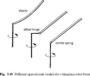that naturally arise are, first, whether these different options are equivalent or what are the important differences in the modelling of flapping motion and hub moments, and second, which is the most appropriate model for flight dynamics applications? We will try to address these questions in the following discussion.

We refer to the analysis of elastic blade flapping at the beginning of Chapter 3 and the series of equations from 3.8 to 3.16, developing the approximate expression for the hub flap moment due to rotor stiffness in the form

The third component due to the lift on the flap arm is O(e3) in the hover and will be neglected. The result given by eqn 3.195 indicates that the hub moment will be out of phase with blade flapping to the extent that any first harmonic aerodynamic load is out of phase with flap. Before examining this phase relationship in a little more detail, we need to explain the inconsistency between Young’s result above in eqn 3.184 and the correct expression given by eqn 3.195. To uncover the anomaly it is necessary to return to the primitive expression for the hub flap moment derived from bending theory (cf. eqn. 3.13):

і 92w 2

F(r, t) — m I -^2 + Q2w

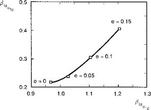
it is assumed that the flap frequency ratio kp and the blade Lock number remain constant throughout. These would normally be set using the corresponding values for the first elastic flap mode frequency and the modal inertia given by eqn 3.11. The values selected are otherwise arbitrary and uses of the offset­spring model in the literature are not consistent in this regard. We chose to draw our comparison for a moderately stiff rotor, with Yp = 1-2 and Sp = 0.2. Figure 3.20 shows a cross-plot of the flap control derivatives for values of offset e extending out to

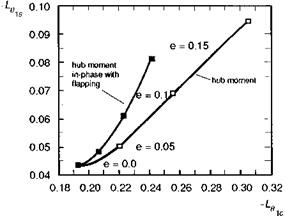
0.15. With e = 0, the flap frequency ratio is augmented entirely with the centre spring; at e = 0.15, the offset alone determines the augmented frequency ratio. The result shows that the rotor flapping changes in character as hinge offset is increased, with the flap/control phase angle decreasing from about 80° for the centre-spring configuration to about 70° with 15% offset. The corresponding roll and pitch hub moment derivatives are illustrated in Fig. 3.21 for the same case. Figure 3.21 shows that over the range of offset-hinge values considered, the primary control derivative increases by 50% while the cross-coupling derivative increases by over 100%. The second curve in Fig. 3.21 shows the variation of the hub moment in phase with the flapping. It can be seen that more than 50% of the change in the primary roll moment derivative is due to the aerodynamic moment from disc flapping in the longitudinal direction. These moments

could not be developed from just the first mode of an elastic blade and are a special feature of large offset-hinge rotors.

The results indicate that there is no simple equivalence between the centre-spring model and the offset-hinge model. Even with Young’s approximation, where the aero­dynamic shear force at the hinge is neglected, the flapping is amplified as shown above. A degree of equivalence, at least for control moments, can be achieved by varying the blade inertia as the offset hinge is increased, hence increasing the effective Lock num­ber, but the relationship is not obvious. Even so, the noticeable decrease in control phasing, coupled with the out-of-phase moments, gives rise to a dynamic behaviour which is not representative of the first elastic flap mode. On the other hand, the appeal of the centre-spring model is its simplicity, coupled with the preservation of the correct phasing between control and flapping and between flapping and hub moment. The ma­jor weakness of the centre-spring model is the crude approximation to the blade shape and corresponding tip deflection and velocity, aspects where the offset-hinge model is more representative.

The selection of parameters for the centre-spring model is relatively straightfor­ward. In the case of hingeless or bearingless rotors, the spring strength and blade inertia are chosen to match the first elastic mode frequency ratio and modal inertia respec­tively. For articulated rotors, the spring strength is again selected to give the correct flap frequency ratio, but now the inertia is changed to match the rotor blade Lock number about the real offset flap hinge.

It needs to be remembered that the rigid blade models discussed above are only approximations to the motion of an elastic blade and specifically to the first cantilever flap mode. In reality, the blade responds by deforming in all of its modes, although the contribution of higher bending modes to the quasi-steady hub moments is usually assumed to be small enough to be neglected. As part of a study of hingeless rotors, Shupe (Refs 3.36 and 3.37) examined the effects of the second flap bending mode on flight dynamics. Because this mode often has a frequency close to three-per-rev, it can have a significant forced response, even at one-per-rev, and Shupe has argued that the inclusion of this effect is important at high speed. This brings us to the domain of aeroelasticity and we defer further discussion until Section 3.4, where we shall explore higher fidelity modelling issues in more detail.

Rotor blades need to lag and twist in addition to flap, and here we discuss briefly the potential contributions of these DoFs to helicopter flight dynamics.

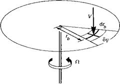
We begin by considering the simple momentum theory applied to the rotor disc element shown in Fig. 3.17. We make the gross assumption that the relationship between the change in momentum and the work done by the load across the element applies locally as well as globally, giving the equations for the mass flow through the element and the thrust differential as shown in eqns 3.161 and 3.162.

dm = pVrb drb df (3.161)

dT = dm 2vi (3.162)

Using the two-dimensional blade element theory, these can be combined into the form

2b ^2pa°c (9UT + UtUp) drb df 2 = 2ргь (V + (ki – )2) 1 ki drb df

(3.163)

Integrating around the disc and along the blades leads to the solution for the mean uniform component of inflow derived earlier. If, instead of averaging the load around the disc, we apply the momentum balance to the one-per-rev components of the load and inflow, then expressions for the non-uniform inflow can be derived. Writing the first harmonic inflow in the form

Xi = X0 + rb(Mc cos ф + Xs sin ф) (3.164)

eqn 3.163 can be expanded to give a first harmonic balance which, in hover, results in the expressions

where the F loadings are given by eqns 3.92 and 3.93. These one-per-rev lift forces are closely related to the aerodynamic moments at the hub in the non-rotating fuselage frame – the pitching moment Сма and the rolling moment Cpa, i. e.,

2CMa _3 f (1)

a0 S = 8 F1c

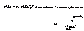
These hub moments are already functions of the non-uniform inflow distributions; hence, just as with the rotor thrust and the uniform inflow, we find that the moments are reduced by a similar moment deficiency factor

CLa = C1 CLaQS (3.169)

(3.170)

(3.171)

in hover, with typical value 0.6, and

1

1 1 00£

1 + 8n

in forward flight, with typical value of 0.8 when д = 0.3. In hover, the first harmonic inflow components given by eqns 3.165 and 3.166 can be expanded as

Ms = C1-^-(91S + в1с + p)

16A0

As the rotor blade develops an aerodynamic moment, the flowfield responds with the linear, harmonic distributions derived above. The associated deficiency factors have often been cited as the cause of mismatches between theory and test (Refs 3.9,3.22­3.29), and there is no doubt that the resulting overall effects on flight dynamics can be significant. The assumptions are fragile however, and the theory can, at best, be regarded as providing a very approximate solution to a complex problem. More recent developments, with more detailed spatial and temporal inflow distributions, are likely to offer even higher fidelity in rotor modelling (see Pitt and Peters, Ref 3.26, and the series of Peters’ papers from 1983, Refs 3.27-3.29).

The inflow analysis outlined above has ignored any time dependency other than the quasi-steady effects and harmonic variations. In reality, there will always be a transient lag in the build-up or decay of the inflow field; in effect, the flow is a dynamic element in its own right. An extension of momentum theory has also been made to include the dynamics of an ‘apparent’ mass of fluid, first by Carpenter and Fridovitch in 1953 (Ref. 3.30). To introduce this theory, we return to axial flight; Carpenter and Fridovitch suggested that the transient inflow could be taken into account by including an accelerated mass of air occupying 63.7% of the air mass of the circumscribed sphere of the rotor. Thus, we write the thrust balancing the mass flow through the rotor to include an apparent mass term

inflow is therefore very rapid, according to simple momentum considerations, but this estimate is clearly a linear function of the ‘apparent mass’. Since this early work, the concept of dynamic inflow has been developed by a number of researchers, but it is the work of Peters, stemming from the early Ref. 3.23 and continuing through to Ref. 3.29, that has provided the most coherent perspective on the subject from a fluid mechanics standpoint. The general formulation of a 3-DoF dynamic inflow model can be written in the form

The matrices M and L are the apparent mass and gain functions respectively; Ct , Cl and Cm are the thrust, rolling and pitching aerodynamic moment perturbations inducing the uniform and first harmonic inflow changes. The mass and gain matrices can be derived from a number of different theories (e. g., actuator disc, vortex theory). In the most recent work, Peters has extended the modelling to an unsteady three­dimensional finite-state wake (Ref. 3.29) which embraces the traditional theories of Theordorsen and Lowey (Ref. 3.31). Dynamic inflow will be discussed again in the context of stability and control derivatives in Chapter 4, and the reader is referred to Refs 3.28 and 3.29 for full details of the aerodynamic theory.

Before discussing additional rotor dynamic DoFs and progressing on to other helicopter components, we return to the centre-spring model for a further examination of its merits as a general approximation.

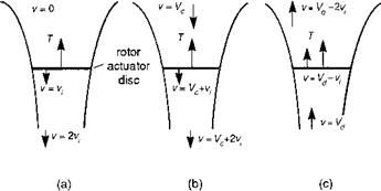
Figures 3.12 (a)-(c) illustrate the flow states for the rotor in axial motion, i. e., when the resultant flow is always normal to the rotor disc, corresponding to hover, climbing or descending flight. The flow is assumed to be steady, inviscid and incompressible with a well-defined slipstream between the flowfield generated by the actuator disc (i. e., streamtube extending to infinity) and the external flow. Physically, this last condition is violated in descending flight when the flow is required to turn back on itself; we shall return to this point later. A further assumption we will make is that the pressure in the far wake returns to atmospheric. These assumptions are discussed in detail by Bramwell (Ref. 3.6) and Johnson (Ref. 3.7), and will not be laboured here. The simplest theory that allows us to derive the relationship between rotor thrust and torque and the rotor inflow is commonly known as momentum theory, utilizing the conservation laws of mass, momentum and energy. Our initial theoretical development will be based on the so-called global momentum theory, which assumes that the inflow is uniformly distributed over the rotor disc. Referring to Fig. 3.12, we note that T is the rotor thrust, v the velocity at various stations in the streamtube, vi the inflow at the disc, Vc the climb velocity and Vd the rotor descent velocity.

First, we shall consider the hover and climb states (Figs 3.12(a), (b)). If m is the mass flow rate (constant at each station) and Ad the rotor disc area, then we can write the mass flow through the rotor as

The rate of change of momentum between the undisturbed upstream conditions and the far wake can be equated to the rotor loading to give

t = m(Vc + vi) – tn Vc = m vi(З.120) where Vf^ is the induced flow in the fully developed wake.

The change in kinetic energy of the flow can be related to the work done by the rotor (actuator disc); thus

t (Vc + vi„) = іm (Vc + vi„)2 – іmvC = 2m (2^ + v?.) (3.121)

From these relationships we can deduce that the induced velocity in the far wake is accelerated to twice the rotor inflow, i. e.,

	(3.122)

The expression for the rotor thrust can now be written directly in terms of the conditions at the rotor disc; hence

T = 2 pAd (Vc + vi )vi

Writing the inflow in normalized form

(3.124)

we may express the hover-induced velocity (with Vc = 0) in terms of the rotor thrust coefficient, Ct, i. e.,

(3.125)

v ihover

The inflow in the climb situation can be written as

Ct

2(Mc + ki)

or, derived from the positive solution of the quadratic

2

kih = (Mc + ki )ki

as

where

_Vl a r

The case of vertical descent is more complicated. Strictly, the flow state satisfies the requirements for the application of momentum theory only in conditions where the wake is fully established above the rotor and the flow is upwards throughout the streamtube. This rotor condition is called the windmill brake state, in recognition of the similarity to a windmill, which extracts energy from the air (Fig. 3.12(c)). The work done by the rotor on the air is now negative and, following a similar analysis to that for the climb, the rotor thrust can be written as

T — 2pAd(Vd – vі)vi (3.130)

The inflow at the disc in the windmill brake state can therefore be written as

where

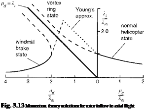The ‘physical’ solutions of eqns 3.128 and 3.131 are shown plotted as the full lines in Fig. 3.13. The dashed lines correspond to the ‘unrealistic’ solutions. These solutions include descent rates from hover through to the windmill brake condition, thus encom­passing the so-called ideal autorotation condition when the inflow equals the descent rate. This region includes the vortex-ring condition where the wake beneath the rotor becomes entrained in the air moving upwards relative to the rotor outside the wake and, in turn, becoming part of the inflow above the rotor again. This circulating flow forms a toroidal-shaped vortex which has a very non-uniform and unsteady charac­ter, leading to large areas of high inflow in the centre of the disc and stall outboard. The vortex-ring condition is not amenable to modelling via momentum considerations alone. However, there is evidence that the mean inflow at the rotor can be approximated by a semi-empirical shaping function linking the helicopter and windmill rotor states shown in Fig. 3.13. The linear approximations suggested by Young (Ref. 3.11) are

shown in the figure as the chain dotted lines, and these match the test data gathered by Castles and Gray in the early 1950s (Ref. 3.12) reasonably well. Young’s empirical relationships take the form

bi — 1 + 0 <—id <~1-5Xlh (3.133)

^ = ч (7 – 3- 1-5Xlh < – Ц. d < -2klh (3.134)

One of the important features of approximations like Young’s is that they enable an estimate of the induced velocity in ideal autorotation to be derived. It should be noted that the dashed curve obtained from the momentum solution in Fig. 3.13 never actually crosses the autorotation line. Young’s approximation estimates that the autorotation line is crossed at

— = 1.8 (3.135)

^ih

As pointed out by Bramwell (Ref. 3.6), the rotor thrust in this condition equates to the drag of a circular plate of the same diameter as the rotor, i. e., the rotor is descending with a rate of descent similar to that of a parachute.

Momentum theory in forward flight

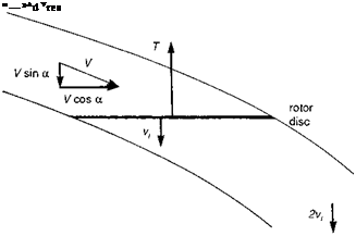
In high-speed flight the downwash field of a rotor is similar to that of a fixed-wing aircraft with circular planform and the momentum approximations for deriving the induced flow at the wing apply (Ref. 3.13). Figure 3.14 illustrates the flow streamtube, with freestream velocity V at angle of incidence a to the disc, and the actuator disc inducing a velocity vi at the rotor. The induced flow in the far wake is again twice the flow at the rotor (wing) and the conservation laws give the mass flux as

(3.136)

and hence the rotor thrust (or wing lift) as

T = riilvi = 2p AdVresvi (3.137)

where the resultant velocity at the rotor is given by

Vr2s = (V cos ad)2 + (V sin ad + vt)2 (3.138)

Normalizing velocities and rotor thrust in the usual way gives the general expression

k = 1 == (3.139)

V[д2 + (ki – Hz )2]

where

and where ad is the disc incidence, shown in Fig. 3.14. Strictly, eqn 3.139 applies to high-speed flight, where the downwash velocities are much smaller than in hover, but it can be seen that the solution also reduces to the cases of hover and axial motion in the limit when h = 0. In fact, this general equation is a reasonable approximation to the mean value of rotor inflow across a wide range of flight conditions, including steep descent, and also provides an estimate of the induced power required.

Summarizing, we see that the rotor inflow can be approximated in hover and high-speed flight by the formulae

showing the dependence on the square root of disc loading in hover, and proportional to disc loading in forward flight.

Between hover and h values of about 0.1 (about 40 knots for Lynx), the mean normal component of the rotor wake velocities is still high, but now gives rise to fairly strong non-uniformities along the longitudinal, or, more generally, the flight axis of the disc. Several approximations to this non-uniformity were derived in the early developments of rotor aerodynamic theory using the vortex form of actuator disc theory (Refs 3.14-3.16). It was shown that a good approximation to the inflow could be achieved with a first harmonic with a linear variation along the disc determined by the wake angle relative to the disc, given by

where

k1cw — k0tan 2 ^ , X <

and the wake angle, x, is given by

where k0 is the uniform component of inflow as given by eqn 3.139.

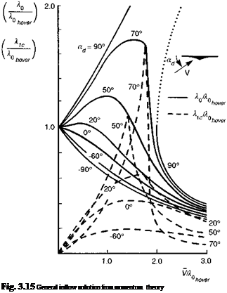The solution of eqn 3.144 can be combined with that of eqn 3.139 to give the results shown in Fig. 3.15 where, again, ad is the disc incidence and Vis the resultant velocity of the free stream relative to the rotor. The solution curves for the (non-physical) vertical descent cases are included. It can be seen that the non-uniform component is approximately equal to the uniform component in high-speed straight and level flight, i. e., the inflow is zero at the front of the disc. In low-speed steep descent, the non­uniform component varies strongly with speed and is also of similar magnitude to the uniform component. Longitudinal variations in blade incidence lead to first harmonic lateral flapping and hence rolling moments. Flight in steep descent is often characterized by high vibration, strong and erratic rolling moments and, as the vortex-ring region is entered, loss of vertical control power and high rates of descent (Ref. 3.17). The

1.0 2.0 horizontal velocity parameter, V cos y/vh

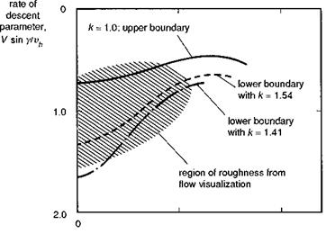simple uniform/non-uniform inflow model given above begins to account for some of these effects (e. g., power settling, Ref. 3.18) but cannot be regarded as a proper representation of either the causal physics or flight dynamics effects; in particular, the dramatic loss of control power caused by the build up of the toroidal vortex ring is not captured by the simple model, and recourse to empiricism is required to model this effect. An effective analysis to predict the boundaries of the vortex-ring state, using momentum theory, was conducted in the early 1970s (Ref. 3.19) and extended in the 1990s using classical vortex theory (Ref. 3.20). Wolkovitch’s results are summarized in Fig. 3.16, showing the predicted upper and lower boundaries as a function of normalized horizontal velocity; the so-called region of roughness measured previously by Drees (Ref. 3.21) is also shown. The parameter k shown on Fig. 3.16 is an empirical constant scaling the downward velocity of the wake vorticity. The lower boundary is set at a value of k < 2, i. e., before the wake is fully contracted, indicating breakdown of the protective tube of vorticity a finite distance below the rotor. Knowledge of the boundary locations is valuable for including appropriate flags in simulation models (e. g., Helisim). Once again though, the simple momentum and vortex theories are inadequate at modelling the flow and predicting flight dynamics within the vortex-ring region. We shall return to this topic in Chapters 4 and 5 when discussing trim and control response.

The momentum theory used to formulate the expressions for the rotor inflow is strictly applicable only in steady flight when the rotor is trimmed and in slowly varying conditions. We can, however, gain an appreciation of the effects of inflow on rotor thrust during manoeuvres through the concept of the lift deficiency function (Ref. 3.7). When the rotor thrust changes, the inflow changes in sympathy, increasing for increasing thrust and decreasing for decreasing thrust. Considering the thrust changes

as perturbations on the mean component, we can write

SCt = 5Cres + (^l)Qs Ski where, from the thrust equation (eqn 3.91)

d Ct a()S

dki ) qs 4

and where the quasi-steady thrust coefficient changes without change in the inflow. Assuming that the inflow changes are due entirely to thrust changes, we can write

5ki = C SCt (3.148)

The derivatives of inflow with thrust have simple approximate forms at hover and in forward flight

Combining these relationships, we can write the thrust changes as the product of a deficiency function and the quasi-steady thrust change, i. e.,

SCT = C ‘SCTqs (3.151)

where

C = , V = 0 (3.152)

1 + 16ki

and

C = V > 0.2 (3.153)

1 + 8v

Rotor thrust changes are therefore reduced to about 60-70% in hover and 80% in the mid-speed range due to the effects of inflow. This would apply, for example, to the thrust changes due to control inputs. It is important to note that these deficiency functions do not apply to the thrust changes from changes in rotor velocities. In particular, when the vertical velocity component changes, there are additional inflow perturbations that lead to even further lift reductions. In hover, the deficiency function for vertical velocity changes is half that due to collective pitch changes, i. e.,

sensitivity of rotors increases strongly from hover to mid speed, but levels out to the constant quasi-steady value at high speed (see discussion on vertical gust response in Chapter 2).

Because the inflow depends on the thrust and the thrust depends on the inflow, an iterative solution is required. Defining the zero function g0 as

g0 = 10 -(2S/2) (3 ‘551

where

Л = p2 + (10 – Pz)2 (3.156)

and recalling that the thrust coefficient can be written as (eqn 3.91)

+ 4 + p2) &t

(3.157)

Newton’s iterative scheme gives

10j+1 = – Ц + fjhj( 10 j)

where

i. e.,

For most flight conditions the above scheme should provide rapid estimates of the inflow at time tj+1 from a knowledge of conditions at time tj. The stability of the algorithm is determined by the variation of the function g0 and the initial value of I0. However, in certain flight conditions near the hover, the iteration can diverge, and the damping constant f is included to stabilize the calculation; a value of 0.6 for f appears to be a reasonable compromise between achieving stability and rapid convergence (Ref. 3.4).

A further approximation involved in the above inflow formulation is the assump­tion that the freestream velocity component normal to the disc (i. e., V sin ad) is the same as pz. This is a reasonable approximation for small flapping angles, and even for the larger angles typical of low-speed manoeuvres the errors are small because of the insensitivity of the inflow to disc incidence (see Fig. 3.15). The approximation is convenient because there is no requirement to know the disc tilt or rotor flapping relative to the shaft to compute the inflow, hence leading to a further simplification in the iteration procedure.

The simple momentum inflow derived above is effective in predicting the gross and slowly varying uniform and rectangular, wake-induced, inflow components. In practice, the inflow distribution varies with flight condition and unsteady rotor loading (e. g., in manoeuvres) in a much more complex manner. Intuitively, we can imagine the inflow varying around the disc and along the blades, continuously satisfying local flow balance conditions and conservation principles. Locally, the flow must respond to local changes in blade loading, so if, for example, there are one-per-rev rotor forces and mo­ments, we might expect the inflow to be related to these. We can also expect the inflow to take a finite time to develop as the air mass is accelerated to its new velocity. Also, the rotor wake is far more complex and discrete than the uniform flow in a streamtube assumption of momentum theory. It is known that local blade-vortex interactions can cause very large local perturbations in blade inflow and hence incidence. These can be sufficient to stall the blade in certain conditions and are important for predicting rotor stall boundaries and the resulting flight dynamics at the flight envelope limits. We shall return to this last topic later in the discussion on advanced, high-fidelity modelling. Before leaving inflow however, we shall examine the theoretical developments needed to improve the prediction of the non-uniform and unsteady components.

The rotor inflow is the name given to the flowfield induced by the rotor at the rotor disc, thus contributing to the local blade incidence and dynamic pressure. In general, the induced flow at the rotor consists of components due to the shed vorticity from all the blades, extending into the far wake of the aircraft. To take account of these effects fully, a complex vortex wake, distorted by itself and the aircraft motion would need to be modelled. We shall assume that for flight dynamics analysis it is sufficient to consider the normal component of inflow, i. e., the rotor-induced downwash. We shall

also make a number of fairly gross assumptions about the rotor and the character of the fluid motion in the wake in order to derive relatively simple formula for the downwash. The use of approximations to the rotor wake for flight dynamics applications has been the subject of two fairly comprehensive reviews of rotor inflow (Refs 3.9, 3.10), which deal with both quasi-static and dynamic effects; the reader is directed towards these works to gain a deeper understanding of the historical development of inflow modelling within the broader context of wake analysis. The simplest representation of the rotor wake is based on actuator disc theory, a mathematical artifact effectively representing a rotor with infinite number of blades, able to accelerate the air through the disc and to support a pressure jump across it. We begin by considering the rotor in axial flight.

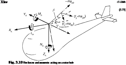Returning to the fundamental frames of reference given in Appendix 3A, in association with Fig. 3.10, we note that the hub forces in the hub-wind frame can be written as

The effective blade incidence angles are given by

a1sw — phw ^1sw + ^1cw + $1sw (3.98)

a1cw — qhw ^1cw ^1sw + ^1cw (3.99)

The foregoing expressions for the rotor forces highlight that in the non-rotating hub – wind-shaft axes system, a multitude of physical effects combine to produce the resul­tants. While the normal force, the rotor thrust, is given by a relatively simple equation, the in-plane forces are very complex indeed. However, some physical interpretation can be made. The F01)^1cw and Fjpeo components are the first harmonics of the product of the lift and flapping in the direction of motion and represent the contribution to X and Y from blades in the fore and aft positions. The terms F^’ and F^ represent the contributions to X and Y from the induced and profile drag acting on the advancing and retreating blades. In hover, the combination of these effects reduces to the simple result that the in-plane contributions from the blade lift forces cancel, and the hub forces are given entirely by the tilt of the rotor thrust vector, i. e.,

Cxw — Ct P1cw (3.100)

Cyw — – Ct hsw (3.101)

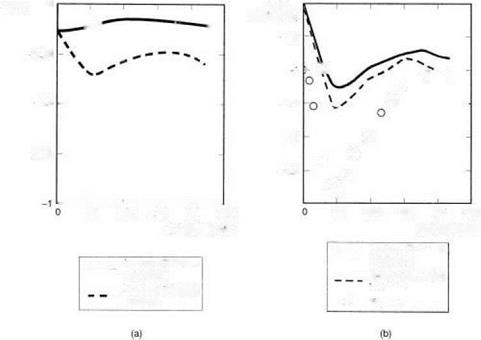
The assumption that the rotor thrust is normal to the disc throughout the flight envelope provides a common approximation in helicopter flight dynamics, effectively ignoring the many small contributions of the blade lift to the rotor in-plane forces given in the above equations. The approximation fails to model many effects however, particularly in lateral trims and dynamics. As an illustration, Fig. 3.11(a) shows a comparison of the rotor Y force in trim as a function of flight speed for the Helisim Bo105; the disc tilt approximation is grossly in error. The corresponding lateral cyclic comparison is shown in Fig. 3.11(b), indicating that the effect of the approximation on lateral trim is actually less significant. The disc tilt approximation is weakest in manoeuvres, particularly for teetering rotors or articulated rotors with small flapping hinge offsets, when the damping moment is dominated by the rotor lateral force rather than the hub moments. The most significant of the 3.90 series of equations is the first, the zeroth harmonic rotor thrust that appears in normalized form in eqn 3.90 itself. This simple equation is one of the most important in helicopter flight dynamics and we will return to it for more discussion when we explore the rotor downwash in the next section. To complete this rather lengthy derivation of the rotor forces and moments, we need to orient the hub-wind force components into shaft axes and derive the hub moments.

Using the transformation matrix derived in the Appendix, Section 3A.4, namely

cos фw — sin фw

sin fw cos fw

we can write the X, Yforces in the shaft axes system aligned along the fuselage nominal plane of symmetry,

(3.103)

Fig. 3.11 Rotor side force and lateral cyclic variations in trimmed flight: (a) rotor side force
(Bo105); (b) lateral cyclic pitch (Bo105)

The rotor hub roll (L) and pitch (M) moments in shaft axes, due to the rotor stiffness effect, are simple linear functions of the flapping angles in MBCs and can be written in the form

Lh = —fKpPu (3.104)

Mh = —N-KpP1C (3.105)

The disc flap angles can be obtained from the corresponding hub-wind values by applying the transformation

The hub stiffness can be written in terms of the flap frequency ratio, i. e.,

K = ($ – 1) IpV2

showing the relationship between hub moment and flap frequency (cf. eqn 3.32). The equivalent Kp for a hingeless rotor can be three to four times that for an articulated rotor, and it is this amplification, rather than any significant difference in the magnitude

of the flapping for the different rotor types, that produces the greater hub moments with hingeless rotors.

Rotor torque

The remaining moment produced by the rotor is the rotor torque and this produces a dominant component about the shaft axis, plus smaller components in pitch and roll due to the inclination of the disc to the plane normal to the shaft. Referring to Fig. 3.10, the torque moment, approximated by the yawing moment in the hub-wind axes, can be obtained by integrating the moments of the in-plane loads about the shaft axis

(3.107)

We can neglect all the inertia terms except the accelerating torque caused by the rotor angular acceleration, hence reducing eqn 3.107 to the form,

(3.108)

where IR is the moment of inertia of the rotor blades and hub about the shaft axis, plus any additional rotating components in the transmission system. Normalizing the torque equation gives

, Nh______________ = 2Cq + Ц J^) й

Іp(йR)2nR3sa0 a0s Y

where

(3.110)

and the aerodynamic torque coefficient can be written as

we may express the rotor torque in the form

where the normalized aerodynamic loads are given by the expressions

г = U T в + UPUT, d = — U T (3.114)

ao

The three components of torque can then be written as

Expanding eqn 3.115 and making further approximations to neglect small terms leads to the final equation for rotor aerodynamic torque, comprising the induced terms formed from the product of force and velocity and the profile torque, namely

The rotor disc tilt relative to the shaft results in components of the torque in the roll and pitch directions. Once again, only one-per-rev roll and pitch moments in the rotating frame of reference will transform through as steady moments in the hub-wind axes. Neglecting the harmonics of rotor torque, we see that the hub moments can therefore be approximated by the orientation of the steady torque through the one-per-rev disc title

Lhq = —f fhc (3.117)

Mhq = QR flu (3.118)

We shall return to the discussion of hub forces and moments later in Section 3.4 and Chapter 4. We still have considerable modelling ground to cover however, not only for the different helicopter components, but also with the main rotor to cover the details of the ‘inner’ dynamic elements. First, we take a closer look at rotor inflow.

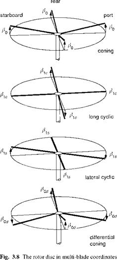
We can introduce a transformation from the individual blade coordinates (IBCs) to the disc coordinates, or multi-blade coordinates (MBCs), as follows:

(3.49)

Once again, the reference zero angle for blade 1 is at the rear of the disc. The MBCs can be viewed as disc mode shapes (Fig. 3.8). The first, во, is referred to as coning – all the blades flap together in a cone. The first two cyclic modes в1с and e1s represent first harmonic longitudinal and lateral disc tilts, while the higher harmonics appear as a disc warping. For Nb = 4, the oddest mode of all is the differential coning, Pod, which can be visualized as a mode with opposite pairs of blades moving in unison, but

in opposition to neighbour pairs, as shown in Fig. 3.8. The transformation to MBCs has not involved any approximation; there are the same number of MBCs as there are IBCs, and the individual blade motions can be completely reconstituted from the MBC motions. There is one other important aspect that is worth highlighting. MBCs are not strictly equivalent to the harmonic coefficients in a Fourier expansion of the blade angle. In general, each blade will be forced and will respond with higher than a one-per-rev component (e. g., two-, three – and four-per-rev), yet with Nb = 3, only first harmonic MBCs will exist; the higher harmonics are then folded into the first harmonics. The real benefit of MBCs emerges when we conduct the coordinate transformation on the uncoupled individual blade eqns 3.34, written in matrix form as
hence forming the MBC equations

Pm + cm ІФ )P’M + Dm ІФ )Pm = Hm ІФ) (3.51)

where the coefficient matrices are derived from the following expressions:

The MBC system described by eqn 3.51 can be distinguished from the IBC system in two important ways. First, the equations are now coupled, and second, the periodic terms in the coefficient matrices no longer contain first harmonic terms but have the lowest frequency content at Nb/2 per-rev (i. e., two for a four-bladed rotor). A common approximation is to neglect these terms, hence reducing eqn 3.51 to a set of ordinary differential equations with constant coefficients that can then be appended to the fuse­lage equations of motion allowing the wide range of linear stationary stability analysis tools to be brought to bear. In the absence of periodic terms, MBC equations take the form

Pm + Cm 0PM + Dm 0Pm = Hm 0(f) (3.55)

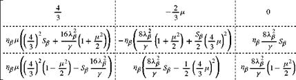
where the constant coefficient matrices can be expanded, for a four-bladed rotor, as shown below:

(3.56)

)

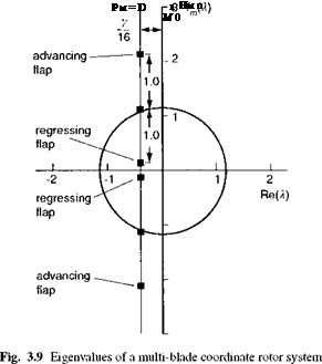
The two modes have been described as the flap precession (or regressing flap mode) and nutation (or advancing flap mode) to highlight the analogy with a gyroscope; both have the same damping factor as the coning mode but their frequencies are widely separated, the precession lying approximately at X – 1) and the nutation well beyond this at (Xe + 1). While the nutation flap mode is unlikely to couple with the fuselage motions, the regressing flap mode frequency can be of the same order as the highest frequency fuselage modes. An often used approximation to this mode assumes that the inertia terms are zero and that the simpler, first-order formulation is adequate for describing the rotor flap as described in Chapter 2 (eqn 2.40). The motion tends to be more strongly coupled with the roll axis because of the lower time constant associated with roll than with pitch motion. The roll to pitch time constants are scaled by the ratio of the roll to pitch moment of inertia, a parameter with a typical value of about 0.25. We shall return to this approximation later in this chapter and in Chapter 5.

The differential coning is of little interest to us, except in the reconstruction of the individual blade motions; each pair of blade exerts the same effective load on the rotor hub, making this motion reactionless. Ignoring this mode, we see that the quasi-steady motion of the coning and cyclic flapping modes can be derived from eqn 3.55 and written in vector-matrix form as

or expanded as

вм = Ape 0 + ApxX + Арыш (3.65)

where the subvectors are defined by

вм = {во, Ріс, Pis} (3.66)

0 ={{0, etw-l eisw 7 eicw } (3.67)

X = {(Д^ — ^0)7 ^1sw 7 Xicw } (3.68)

W = {p’hw 7 qhw 7 Phw 7 qhw } (3.69)

and the coefficient matrices can be written as shown opposite in eqns 3.70, 3.71 and 3.72. Here

1

1 + SP

These quasi-steady flap equations can be used to calculate rotor trim conditions to O(p? ) and also to approximate the rotor dynamics associated with low-frequency fuselage

motions. In this way the concept of flapping derivatives comes into play. These were introduced in Chapter 2 and examples were given in eqns 2.29-2.32; the primary flap control response and damping in the hover were derived as

showing the strong dependence of rotor flap damping on Lock number, compared with the weak dependence of flap response due to both control and shaft angular motion on rotor stiffness. To emphasize the point, we can conclude that conventional rotor types from teetering to hingeless, all flap in much the same way. Of course, a hingeless rotor will not need to flap nearly as much and the pilot might be expected to make smaller control inputs than with an articulated rotor, to produce the same hub moment and hence to fly the same manoeuvre.

The coupled rotor-body motions, whether quasi-steady or with first – or second – order flapping dynamics, are formed from coupling the hub motions with the rotor and driving the hub, and hence the fuselage, with the rotor forces. The expressions for the hub forces and moments in MBC form will now be derived.

Reference to Fig. 3.6 shows that the equation of motion for the blade flap angle в (t) of the ith blade can be obtained by taking moments about the centre hinge with spring strength Kp; thus

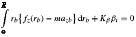(3.18)

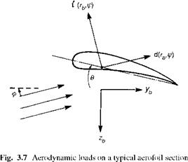
The blade radial distance has now been written with a subscript b to distinguish it from similar variables. We have neglected the blade weight force in eqn 3.18; the mean lift and acceleration forces are typically one or two orders of magnitude higher. We follow the normal convention of setting the blade azimuth angle, ф, to zero at the rear of the disc, with a positive direction following the rotor. The analysis in this book applies to a rotor rotating anticlockwise when viewed from above. From Fig. 3.7, the aerodynamic load fz(rb, t) can be written in terms of the lift and drag forces as

fz = —t cos ф — d sin ф t — dф

where ф is the incidence angle between the rotor inflow and the plane normal to the rotor shaft. We are now working in the blade axes system, of course, as defined in Section 3A.4, where the z direction lies normal to the plane of no-pitch. The acceleration normal to the blade element, azb, includes the component of the gyroscopic effect due to the

rotation of the fuselage and hub, and is given approximately by (see the Appendix, Section 3A.4)

azb ~ rb ^2fi( phw cos fi – qhw sin fi) + (qhw cos fi + phw sin fi) – & в –

(3.20)

The angular velocities and accelerations have been referred to hub-wind axes in this formulation, and hence the subscript hw. Before expanding and reducing the hub moment in eqn 3.18 further, we need to review the range of approximations to be made for the aerodynamic lift force. The aerodynamic loads are in general unsteady, nonlinear and three-dimensional in character; our first approximation neglects these effects, and, in a wide range of flight cases, the approximations lead to a reasonable prediction of the overall behaviour of the rotor. So, our starting aerodynamic assumptions are as follows:

(1) The rotor lift force is a linear function of local blade incidence and the drag force is a simple quadratic function of lift – both with constant coefficients. Neglecting blade stall and compressibility can have a significant effect on the prediction of performance and dynamic behaviour at high forward speeds. Figure 2.10 illustrated the proximity of the local blade incidence to stall particularly at rotor azimuth angles 90° and 180°. Without these effects modelled, the rotor will be able to continue developing lift at low drag beyond the stall and drag divergence boundary, which is clearly unrealistic. The assumption of constant lift curve slope neglects the linear spanwise and one-per-rev timewise variations due to compressibility effects. The former can be accounted for to some extent by an effective rotor lift curve slope, particularly at low speed, but the azimuthal variations give rise to changes in cyclic and collective trim control angles in forward flight, which the constant linear model cannot simulate.

(2) Unsteady (i. e., frequency dependent) aerodynamic effects are ignored. Rotor unsteady aerodynamic effects can be conveniently divided into two problems – one involves the calculation of the response of the rotor blade lift and pitching moment to changes in local incidence, while the other involves the calculation of the unsteady local incidence due to the time variations of the rotor wake velocities. Both require additional DoFs to be taken into account. While the unsteady wake effects are

accounted for in a relatively crude but effective manner through the local/dynamic inflow theory described in this section, the time-dependent developments of blade lift and pitching moment are ignored, resulting in a small phase shift of rotor response to disturbances.

(3) Tip losses and root cut-out effects are ignored. The lift on a rotor blade reduces to zero at the blade tip and at the root end of the lifting portion of the blade. These effects can be accounted for when the fall-off is properly modelled at the root and tip, but an alternative is to carry out the load integrations between an effective root and tip. A tip loss factor of about 3% R is commonly used, while integrating from the start of the lifting blade accounts for most of the root loss. Both effects are small and accounts for only a few per cent of performance and response. Including them in the analysis increases the length of the equations significantly however, and can obscure some of the more significant effects. In the analysis that follows, we therefore omit these loss terms, recognizing that to achieve accurate predictions of power, for example, they need to be included.

(4) Non-uniform spanwise inflow distribution is neglected. The assumption

of uniform inflow is a gross simplification, even in the hover, of the complex effects of the rotor wake, but provides a very effective approximation for predicting power and thrust. The use of uniform inflow stems from the assumption that the rotor is designed to develop minimum induced drag, and hence has ideal blade twist. In such an ideal case, the circulation would be constant along the blade span, with the only induced losses emanating from the tip and root vortices. Ideal twist, for a constant chord blade, is actually inversely proportional to radius, and the linear twist angles of O (10°), found on most helicopters, give a reasonable, if not good, approximation to the effects of ideal twist over the outer lifting portion of the blades. The actual non-uniformity of the inflow has a similar shape to the bound circulation, increasing outboard and giving rise to an increase in drag compared with the uniform inflow theory. The blade pitch at the outer stations of a real blade will need to be increased relative to the uniform inflow blade to produce the same lift. This increase produces more lift inboard as well, and the resulting comparison of trim control angles may not be significantly different.

(5) Reversed flow effects are ignored. The reversed flow region occupies

the small disc inboard on the retreating side of the disc, where the air flows over the blades from trailing to leading edge. Up to moderate forward speeds, the extent of this region is small and the associated dynamic pressures low, justifying its omission from the analysis of rotor forces. At higher speeds, the importance of the reversed flow region increases, resulting in an increment to the collective pitch required to provide the rotor thrust, but decreasing the profile drag and hence rotor torque.

These approximations make it possible to derive manageable analytic expressions for the flapping androtor loads. Referring to Fig. 3.7, the aerodynamic loads can be written in the form

where

We have made the assumption that the blade profile drag coefficient S can be written in terms of a mean value plus a thrust-dependent term to account for blade incidence changes (Refs 3.6,3.7). The non-dimensional in-plane and normal velocity components can be written as

Ut = гь(1 + rnxв) + д sin f (3.24)

Up = (д1 – Ло – вд cos f) + rb(Vy – в’ – Л1) (3.25)

We have introduced into these expressions a number of new symbols that need definition:

The velocities uhw, vkw and wbw are the hub velocities in the hub-wind system, oriented relative to the aircraft x-axis by the relative airspeed or wind direction in the x-y plane. в is the blade flap angle and 9 is the blade pitch angle. The fuselage angular velocity components in the blade system, normalized by Q R, are given by

Vx = Phw cos fі – qhw sin fі

Vy = phw sin fi + qhw cos fi (3.29)

The downwash, Л, normal to the plane of the rotor disc, is written in the form of a uniform and linearly varying distribution

vi

Л == Л0 + M(f )rb (3.30)

Q R

This simple formulation will be discussed in more detail later in this chapter.

We can now develop and expand eqn 3.18 to give the second-order differential equation of flapping motion for a single blade, with the prime indicating differentiation with respect to azimuth angle f:

derived directly from the hub stiffness and the flap moment of inertia Ip

where ao is the constant blade lift curve slope, p is the air density and c the blade chord.

Writing the blade pitch angle 9 as a combination of applied pitch and linear twist, in the form

9 = 9 p + rb9tw (3.33)

we may expand eqn 3.31 into the form

p” + fp’ Yp’ + (^2p + YH cos fife) Pi =

2((Tw + – w) cos fi – (vw – j sin ftj

+ Y f9p9p + f9tw9tw + fX(Hz — X0) + frn(®y — X1^ (3.34)

where the aerodynamic coefficients, f, are given by the expressions

These aerodynamic coefficients have been expanded up to O (h2); neglecting higher order terms incurs errors of less than 10% in the flap response below h of about 0.35. In Chapter 2, the Introductory Tour of this subject, we examined the solution of eqn 3.34 at the hover condition. The behaviour was discussed in some depth there, and to avoid duplication of the associated analysis we shall restrict ourselves to a short resume of the key points from the material in Chapter 2.

lag, but even the Lynx, with its moderately stiff rotor, has about 80° of lag between cyclic pitch and flap. The phase lag is proportional to the stiffness number (effectively the ratio of stiffness to blade aerodynamic moment), given by

(3)

There is a fundamental rotor resistance to fuselage rotations, due to the aerodynamic damping and gyroscopic forces. Rotating the fuselage with a pitch (q) or roll (p) rate leads to a disc rotation lagged behind the fuselage motion by a time given approximately by (see eqn 2.43)

Hence the faster the rotorspeed, or the lighter the blades, for example, the higher is the rotor damping and the faster is the disc response to control inputs or fuselage motion.

(4) The rotor hub stiffness moment is proportional to the product of the spring strength and the flap angle; teetering rotors cannot therefore produce a hub moment, and hingeless rotors, as on the Bo105 and the Lynx, can develop hub moments about four times those for typical articulated rotors.

(5) The increased hub moment capability of hingeless rotors transforms into increased control sensitivity and damping and hence greater responsiveness at the expense of greater sensitivity to extraneous inputs such as gusts. The control power, or final steady-state rate per degree of cyclic, is independent of rotor stiffness to first order, since it is derived from the ratio of control sensitivity to damping, both of which increase in the same proportion with rotor stiffness.

(6) The flapping of rotors with Stiffness numbers up to about 0.3 is very similar – e. g., approximately 1 ° flap for 1 ° cyclic pitch.

The behaviour of a rotor with Nb blades will be described by the solution of a set of uncoupled differential equations of the form eqn 3.34, phased relative to each other. However, the wake and swash plate dynamics will couple implicitly the blade dynam­ics. We return to this aspect later, but for the moment, assume a decoupled system. Each equation has periodic coefficients in the forward flight case, but is linear in the flap DoFs (once again ignoring the effects of wake inflow). In Chapter 2, we examined the hover case and assumed that the blade dynamics were fast relative to the fuselage motion, hence enabling the approximation that the blade motion was essentially pe­riodic with slowly varying coefficients. The rotor blades were effectively operating in two timescales, one associated with the rotor rotational speed and the other asso­ciated with the slower fuselage motion. Through this approximation, we were able to deduce many fundamental facets of rotor behaviour as noted above. It was also highlighted that the approximation breaks down when the frequencies of the rotor and fuselage modes approached one another, as can happen, for example, with hingeless rotors. This quasi-steady approximation can be approached from a more general per­spective in the forward flight case by employing the so-called multi-blade coordinates (Refs 3.4, 3.8).

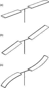
The mechanism of cyclic blade flapping provides indirect control of the direction of the rotor thrust and the rotor hub moments (i. e., the pilot has direct control only of blade pitch), hence it is the primary source of manoeuvre capability. Blade flap retention ar­rangements are generally of three kinds – teetering, articulated and hingeless, or more generally, bearingless (Fig. 3.4). The three different arrangements can appear very con­trasting, but the amplitude of the flapping motion itself, in response to gusts and control inputs, is very similar. The primary difference lies in the hub moment capability. One of the key features of the Helisim model family is the use of a common analogue model for all three types – the so-called centre-spring equivalent rotor (CSER). We need to exam­ine the elastic motion of blade flapping to establish the fidelity of this general approxi­mation. The effects of blade lag and torsion dynamics are considered later in this section.

Blade flapping dynamics – introduction

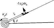
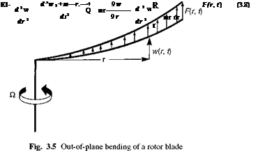
We begin with a closer examination of the hingeless rotor. Figure 3.5 illustrates the out-of-plane bending, or flapping, of a typical rotating blade cantilevered to the rotor

hub. Using the commonly accepted engineer’s bending theory, the linearized equation of motion for the out-of-plane deflexion w(r, t) takes the form of a partial differential equation in space radius r and time t, and can be written (Ref. 3.5) as

where EI(r) and m(r) are the blade radial stiffness and mass distribution functions and Q is the rotorspeed. The function F (r, t) represents the radial distribution of the time – varying aerodynamic load, assumed here to act normal to the plane of rotation. As in the case of a non-rotating beam, the solution to eqn 3.8 can be written in separated variable form, as the summed product of mode shapes Sn(r) and generalized coordinates Pn(t), i. e.,

where P1 is given by eqn 3.10 with n = 1. Equations 3.10 and 3.16 provide the so­lution for the first mode of flapping response of a rotor blade. How well this will approximate the complete solution for the blade response depends on the form of the aerodynamic load F(r, t). From eqns 3.10 and 3.12, if the loading can be approximated by a distribution with the same shape as S1, then the first mode response would suffice. Clearly this is not generally the case, but the higher mode responses can be expected to be less and less significant. It will be shown that the first mode frequency is always close to one-per-rev, and combined with the predominant forcing at one-per-rev the first flap mode generally does approximate the zero and one-per-rev blade dynamics and hub moments reasonably well, for the frequency range of interest in flight dynam­ics. The approximate model used in the Helisim formulation simplifies the first mode formulation even further to accommodate teetering and articulated rotors as well. The articulation and elasticity is assumed to be concentrated in a hinged spring at the centre of rotation (Fig. 3.6), otherwise the blade is straight and rigid; thus

r

Fig. 3.6 The centre-spring equivalent rotor analogue

Such a shape, although not orthogonal to the elastic modes, does satisfy eqn 3.11 in a distributional sense. The centre-spring model is used below to represent all classes of retention system and contrasts with the offset-hinge and spring model used in a number of other studies. In the offset-hinge model, the hinge offset is largely determined from the natural frequency whereas in the centre-spring model, the stiffness is provided by the hinge spring. In many ways the models are equivalent, but they differ in some important features. It will be helpful to derive some of the characteristics of blade flapping before we compare the effectiveness of the different formulations. Further discussion is therefore deferred until later in this section.

In the following four subsections, analytic expressions for the forces and moments on the various helicopter components are derived. The forces and moments are referred to a system of body-fixed axes centred at the aircraft’s centre of gravity/mass, as illustrated in Fig. 3.1. In general, the axes will be oriented at an angle relative to the principal axes of inertia, with the x direction pointing forward along some convenient fuselage reference line. The equations of motion for the six fuselage DoFs are assembled by applying Newton’s laws of motion relating the applied forces and moments to the resulting translational and rotational accelerations. Expressions for the inertial velocities and accelerations in the fuselage-fixed axes system are derived in Appendix Section 3A.1, with the resulting equations of motion taking the classic form as given below.

(3.1) (3.2) (3.3)

hxp = (Iyy — Izz) qr + Ixz (r + pq) + l

Iyyq = (Izz — Ixx) rp + Ixz (r2 — p2) + M Izzr = (Ixx — Iyy) pq + Ixz( p — qr) + N

where u, v and w and p, q and r are the inertial velocities in the moving axes system; ф, 9 and ф are the Euler rotations defining the orientation of the fuselage axes with respect to earth and hence the components of the gravitational force. Ixx, Iyy, etc., are the fuselage moments of inertia about the reference axes and Ma is the aircraft mass. The external forces and moments can be written as the sum of the contributions from the different aircraft components; thus, for the rolling moment

L = LR + LTR + L f + Ltp + Lfn (3.7)

where the subscripts stand for: rotor, R; tail rotor, TR; fuselage, f; horizontal tailplane, tp; and vertical fin, fn.

In Chapters 4 and 5, we shall be concerned with the trim, stability and response solutions to eqns 3.1-3.6. Before we can address these issues we need to derive the expressions for the component forces and moments. The following four sections con­tain some fairly intense mathematical analyses for the reader who requires a deeper understanding of the aeromechanics of helicopters. The modelling is based essentially on the DRA’s first generation, Level 1 simulation model Helisim (Ref. 3.4).

A few words on notation may be useful before we begin. First, the main rotor analysis is conducted in shaft axes, compared with the rotor-aligned, no-flapping or no­feathering systems. Appendix Section 3A.5 gives a comparison of some expressions in the three systems. Second, the reader will find the same variable name used for different states or parameters throughout the chapter. While the author accepts that there is some risk of confusion here, this is balanced against the need to maintain a degree of conformity with traditional practice. It is also expected that the serious reader of Chapters 3, 4 and 5 will easily cope with any potential ambiguities. Hence, for example, the variable r will be used for rotor radial position and aircraft yaw rate; the variable в will be used for flap angle and fuselage sideslip angle; the variable w will be used for blade displacement and aircraft inertial velocity along the z direction. A third point, and this applies more to the analysis of Chapters 4 and 5, relates to the use of capitals or lowercase for trim and perturbation quantities. For the work in the later modelling chapters we reserve capitals, with subscripts e (equilibrium), for trim states and lowercase letters for perturbation variables in the linear analysis. In

Chapter 3, where, in general, we will be dealing with variables from a zero reference, the conventional lowercase nomenclature is adopted. Possible ambiguities arise when comparing analysis from Chapters 3, 4 and 5, although the author believes that the scope for confusion is fairly minimal.

It is beyond dispute that the observed behaviour of aircraft is so complex and puzzling that, without a well developed theory, the subject could not be treated intelligently. Theory has at least three useful functions;

a) it provides a background for the analysis ofactual occurrences,

b) it provides a rational basis for the planning of experiments and tests, thus securing economy ofeffort,

c) it helps the designer to design intelligently.

Theory, however, is never complete, final or exact. Like design and con­struction it is continually developing and adapting itself to circumstances.

(Duncan 1952)

3.1 Introduction and Scope

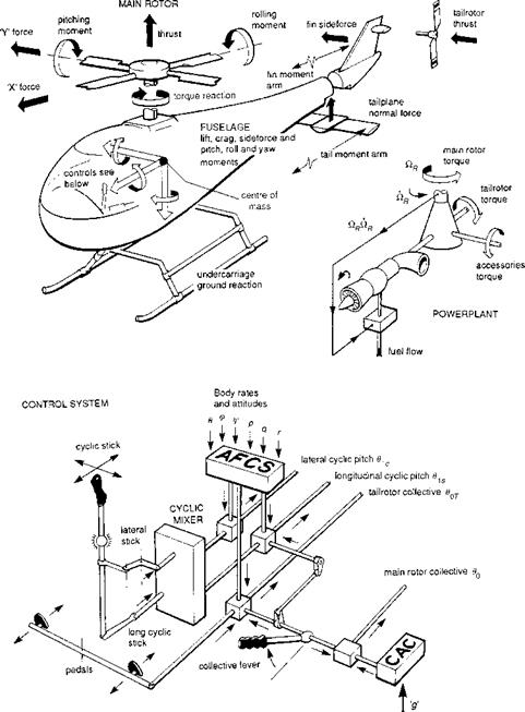
The attributes of theory described by Duncan in this chapter’s guiding quote have a ring of eternal validity to them. With today’s perspective we could add a little more. Theory helps the flying qualities engineer to gain a deep understanding of the behaviour of flight and the limiting conditions imposed by the demands of flying tasks, hence providing insight and stimulating inspiration. The classic text by Duncan (Ref. 3.1) was directed at fixed-wing aircraft, of course. Describing the flight behaviour of the helicopter presents an even more difficult challenge to mathematical modelling. The vehicle can be viewed as a complex arrangement of interacting subsystems, shown in component form in Fig. 3.1. The problem is dominated by the rotor and this will be reflected by the attention given to this component in the present chapter. The rotor blades bend and twist under the influence of unsteady and nonlinear aerodynamic loads, which are themselves a function of the blade motion. Figure 3.2 illustrates this aeroelastic problem as a feedback system. The two feedback loops provide incidence perturbations due to blade (and fuselage) motion and downwash, which are added to those due to atmospheric disturbances and blade pitch control inputs. The calculation of these two incidence perturbations dominates rotor modelling and hence features large in this chapter. For the calculation of aerodynamic loads, we shall be concerned with the blade motion relative to the air and hence the motion of the hub and fuselage as well as the motion of the blades relative to the hub. Relative motion will be a recurring theme in this chapter, which brings into focus the need for common reference frames. This subject is given separate treatment in the appendix to this chapter, where the various axes transformations required to derive the relative motion are set down. Expressions for the accelerations of the fuselage centre of gravity and a rotor blade element are

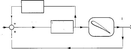
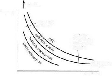Fig. 3.2 Rotor blade aeroelasticity as a feedback problem

derived in the Appendix, Sections 3A.1 and 3A.4, respectively. Rotor blades operate in their own wake and that of their neighbour blades. Modelling these effects has probably consumed more research effort in the rotary-wing field than any other topic, ranging from simple momentum theory (Ref. 3.2) to three-dimensional flowfield solutions of the viscous fluid equations (Ref. 3.3).

The modelling requirements of blade motion and rotor downwash or inflow need to be related to the application. The terms downwash and inflow are used synony­mously in this book; in some references the inflow includes components of free stream flow relative to the rotor, and not just the self-induced downwash. The rule of thumb, highlighted in Chapter 2, that models should be as simple as possible needs to be borne in mind. We refer back to Fig. 2.14 in the Introductory Tour, reproduced here in modified form (Fig. 3.3), to highlight the key dimensions – frequency and amplitude. In flight dynamics, a heuristic rule of thumb, which we shall work with, states that the

vibrabon

frequency

rotor modes aclivatcd

non Imeat aerodynamics and Etmclural dynamics

equi-rssponse contour

amplitude

modelled frequency range in terms of forces and moments needs to extend to two or three times the range at which normal pilot and control system activity occurs. If we are solely concerned with the response to pilot control inputs for normal (correspond­ing to gentle to moderate actions) frequencies up to about 4 rad/s, then achievement of accuracy out to about 10 rad/s is probably good enough. With high gain feedback control systems that will be operating up to this latter frequency, modelling out to 25-30 rad/s may be required. The principal reason for this extended range stems from the fact that not only the controlled modes are of interest, but also the uncontrolled modes, associated with the rotors, actuators and transmission system, that could poten­tially lose stability in the striving to achieve high performance in the primary control loops. The required range will depend on a number of detailed factors, and some of these will emerge as we examine model fidelity in this and the later chapters. With respect to amplitude, the need to model gross manoeuvres defines the problem; in other words, the horizontal axis in Fig. 3.3 extends outwards to the boundary of the operational flight envelope (OFE).

It is convenient to describe the different degrees of rotor complexity in three levels, differentiated by the different application areas, as shown in Table 3.1.

Appended to the fuselage and drive system, basic Level 1 modelling defines the conventional six degree of freedom (DoF) flight mechanics formulation for the fuse­lage, with the quasi-steady rotor taking up its new position relative to the fuselage instantaneously. We have also included in this level the rotor DoFs in so-called multi­blade coordinate form (see Section 3.2.1), whereby the rotor dynamics are consolidated as a disc with coning and tilting freedoms. Perhaps the strongest distinguishing feature of Level 1 models is the analytically integrated aerodynamic loads giving closed form

expressions for the hub forces and moments. The aerodynamic downwash representa­tion in our Level 1 models extends from simple momentum to dynamic inflow.

The analysis of flight dynamics problems through modelling is deferred until Chapters 4 and 5. Chapter 3 deals with model building. For the most part, the model elements are derived from approximations that allow analytic formulations. In this sense, the modelling is far from state of the art, compared with current standards of simulation modelling. This is particularly true regarding the rotor aerodynamics, but the so-called Level 1 modelling described in this chapter is aimed at describing the key features of helicopter flight and the important trends in behaviour with varying design parameters. In many cases, the simplified analytic modelling approximates reality to within 20%, and while this would be clearly inadequate for design purposes, it is ideal for establishing fundamental principles and trends.

There are three sections following. In Section 3.2, expressions for the forces and moments acting on the various components of the helicopter are derived; the main rotor, tail rotor, fuselage and empennage, powerplant and flight control system are initially considered in isolation, as far as this is possible. In Section 3.3, the combined forces and moments on these elements are assembled with the inertial and gravitational forces to form the overall helicopter equations of motion.

Section 3.4 of this chapter takes the reader briefly beyond the realms of Level 1 modelling to the more detailed and higher fidelity blade element and aeroelastic rotor formulations and the complexities of interactional aerodynamic modelling. The flight regimes where this, Level 2, modelling is required are discussed, and results of the kind of influence that aeroelasticity and detailed wake modelling have on flight dynamics are presented.

This chapter has an appendix concerned with defining the motion of the aircraft and rotor in terms of different axes systems as frames of reference. Section 3A.1 de­scribes the inertial motion of an aircraft as a rigid body free to move in three translational and three rotational DoFs. Sections 3A.2 and 3A.3 develop supporting results for the orientation of the aircraft and the components of the gravitational force. Sections 3A.4 and 3A.5 focus on the rotor dynamics, deriving expressions for the acceleration and velocity of a blade element and discussing different axes systems used in the literature for describing the blade motion.